RNA-Seq - Genetic Diversity Centre (GDC)

Learning Objectives

◇ Learn how RNA-Seq works and what technologies it uses.
◇ Understand what RNA-Seq can tell us about biology and how it’s used in research.
◇ Get to know how RNA-Seq experiments are planned and how samples are prepared.
◇ Learn the basics of finding genes that are expressed differently between samples (DEG analysis).

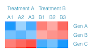
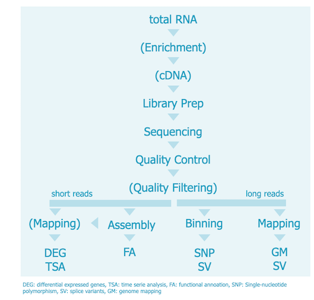
RNA-Seq is a sequencing technique used to study RNA molecules in a biological sample. Common applications include transcriptional (expression) profiling, differential gene expression (DEG) analysis, RNA editing, and even SNP identification. With long-read sequencing technologies (e.g., PacBio, ONT), additional insights such as transcript isoform detection become possible.

Tip

RNA-Seq experiments are powerful if well designed but limited if not. The within sample variations has to be low or the number of replicates (very) high if you want to trust in the results of your differential expression study.

In the exercises, we will focus on identifying differentially expressed genes. While many methods exist for DEG analysis, there is no consensus on a single best workflow. For a comprehensive overview, see Costa-Silva et al. (2017).

Workflow

Quality Control

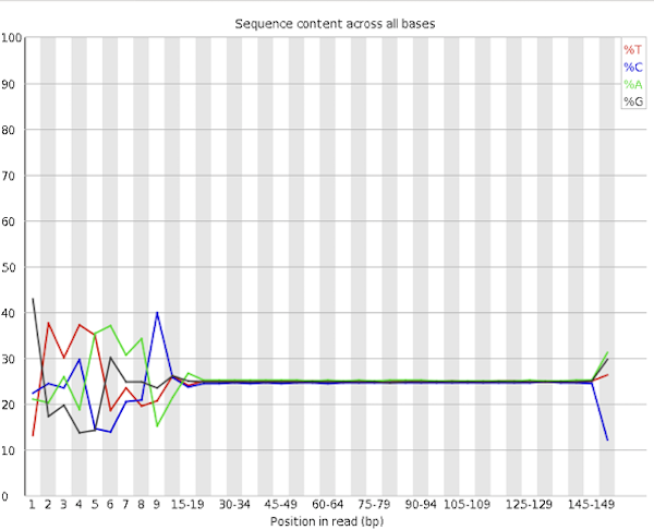
Content Bias - Depending on the method used to prepare the library, RNA-Seq datasets often exhibit a noticeable bias in sequence composition at the beginning of the reads (typically the first ~12 bases). This bias originates from the random priming step during library construction. Ideally, all hexamer primers would bind with equal efficiency, but this is not the case in practice.

Although trimming the reads can remove this bias from QC reports visually, it does not address the underlying issue — and doing so may be misleading. While the QC warning is valid, in most cases there is little that can or should be done to correct this bias directly.

Workflow

Degradation - RNA is inherently unstable and degrades quickly, especially during extraction and handling. Degradation leads to an abundance of short fragments, which is a common feature of RNA-Seq datasets. Preventing degradation requires careful sample handling and the use of RNase-free materials. Proper sample preparation is critical to maintain RNA integrity and minimize fragmentation.

Contaminants - When extracting RNA, it is not just messenger RNA (mRNA) that is isolated; other RNA species are also often captured, such as ribosomal RNA (rRNA), which can dominate the library. Therefore, it is important to choose the appropriate tissue and use enrichment or depletion steps (e.g. poly-A selection or rRNA depletion) to focus the analysis on mRNA. Some library preparation kits include these steps as standard. During quality control (QC), also look out for adapter contamination, which can arise from leftover sequencing adapters in the library.

Duplicate Sequences - High levels of duplicate reads are normal in RNA-Seq datasets. Unlike genomic sequencing, RNA-Seq produces duplicates by design due to the high expression levels of certain transcripts. This is a feature, not a flaw: it reflects true biological enrichment. Therefore, do not remove duplicates, as removing them would distort the gene expression signal.

RNA Integrity

Although standard QC tools such as FastQC can identify technical artefacts (e.g., adaptor contamination, GC bias, or overrepresented sequences), they do not provide a comprehensive assessment of RNA integrity. This is because FastQC evaluates sequencing read quality, not the biological quality of the input RNA.

RNA quality is best assessed before sequencing, using platforms like the Agilent Bioanalyzer or TapeStation, which generate an RNA Integrity Number (RIN). The RIN score reflects the degree of RNA degradation by examining rRNA band patterns (e.g., 28S/18S ratio), and it is widely used to determine whether samples are suitable for RNA-Seq.

For post-sequencing evaluation, especially when pre-sequencing quality control data is unavailable or when degradation may have occurred during library preparation or sequencing, the Transcript Integrity Number (TIN) can be used. TIN is calculated from the read coverage across individual transcripts; low TIN scores suggest degradation or uneven coverage. Plotting principal component analysis (PCA) based on TIN scores, as described by Son et al. (2018), can help visualize and interpret degradation patterns across samples, making it a valuable tool for downstream quality assessment and batch effect detection.

Data Filtering

When we extract RNA from cells, it's not just mRNA that we get (the type required for most RNA-Seq studies); we also collect other types of RNA, particularly ribosomal RNA (rRNA) and transfer RNA (tRNA).

In rapidly growing cells such as HeLa cells, for example, around 80% of the total RNA is rRNA and 15% is tRNA. This means that mRNA makes up only a small portion, around 5%. While these other RNA molecules are important in the cell, they are not usually the focus of RNA-Seq experiments that aim to measure gene expression.

To address this issue, many RNA-Seq library preparation kits incorporate a step to remove rRNA (known as rRNA depletion) or select mRNA only (typically via poly-A selection, which targets the tail of mRNA molecules). However, these methods are not foolproof — some unwanted RNA may still end up in your data.

That’s why it's important to screen your sequence reads after sequencing to check for contamination from non-mRNA sources like rRNA, tRNA, or even genomic DNA. One helpful tool for this is FastQ Screen, which lets you see what kinds of sequences are in your dataset and how much of your data might come from unwanted sources. If necessary, you can filter out those reads before continuing with your analysis.

Statistical Power of RNA-seq Experiments

First, we run a few sample-size power simulation in R using either the R package RNASeqPower or PROPER. Both are Bioconductor packages and can be installed via the BiocManager.

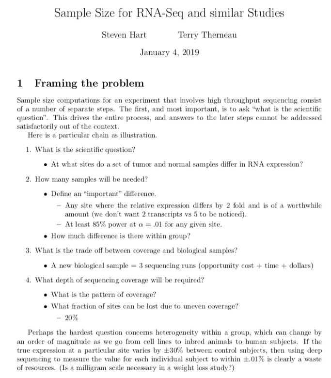
In the (short) manual of RNASeqPower the authors, Steven Hart and Terry Therneau, do an excellent job of describing the problems involved in experimental design of an RNA-Seq experiment.

Hands-on Exercise: Power Analysis in R

In this first hands-on session, we focus on data analysis using R. To begin, you need to download the R script for the exercise. You have two options:

a. Using the terminal (e.g., with curl or wget) to download the script to your local system and then open it in RStudio.

b. Using R (RStudio) directly to both download and open the script within the R environment.

Feel free to choose the method you prefer—or try both to familiarize yourself with the different approaches.

(a) Terminal Approach (Local Shell)

## Working Directory
mkdir ${HOME}/GDA/RNASeq
cd ${HOME}/GDA/RNASeq

## Get R script via terminal
#curl -O https://www.gdc-docs.ethz.ch/GeneticDiversityAnalysis/GDA/scripts/PowerAnalysis_V02.R
curl -O https://www.gdc-docs.ethz.ch/GeneticDiversityAnalysis/GDA/scripts/PowerAnalysis_V03.R
# An alternative to `curl`:
# wget "https://www.gdc-docs.ethz.ch/GeneticDiversityAnalysis/GDA/scripts/PowerAnalysis_V03.R"

Once downloaded, open the script PowerAnalysis_V03.R in RStudio to start the exercise.

(b) RStudio Approach (Within R Console)

This approach allows you to manage everything from within R itself.

## Check your current working directory
getwd()

## Optionally, create and set a working directory
dir.create("RNASeq")            # Similar to 'mkdir'
setwd("RNASeq")                 # Switch to this directory

To download the script from within R, we use the wget() function from the HelpersMG package:

## Install HelpersMG if not already installed
if (!requireNamespace("HelpersMG", quietly = TRUE)) {
  install.packages("HelpersMG")
}

## Load the package
library(HelpersMG)

## Download the R script
#wget("https://www.gdc-docs.ethz.ch/GeneticDiversityAnalysis/GDA/scripts/PowerAnalysis_V02.R")
wget("https://www.gdc-docs.ethz.ch/GeneticDiversityAnalysis/GDA/scripts/PowerAnalysis_V03.R")

## Open the script for editing
file.edit("PowerAnalysis.R")

The Value of This Exercise

While the practical value of power analysis can be debated in some contexts, running these simulations is an excellent way to understand the impact of biological replicates on RNA-seq experiments. Therefore, it’s essential that you don't just copy and paste the code. Take the time to read, understand, and reflect on what each step is doing—you’ll gain a much deeper insight into experimental design and statistical power.

RNA-Seq Data Analysis with DESeq2

Hands-on Exercise: Differential Expression Analysis in R

🔍 Special thanks to Heidi E.L. Tschanz-Lischer

Objective

In this hands-on exercise, you'll perform a differential gene expression analysis using RNA-Seq data from newborn (N), juvenile (J), and adult (A) mice. For each life stage, one female and one male sample were sequenced.

We will:

Load the count data (count table)
Define the sample design
Normalize and transform the data
Visualize sample clustering
Identify differentially expressed genes (DEGs)
Explore specific genes using plotCounts
Link gene IDs to gene names using biomaRt

1. Download and Import the Count Table

# Download the count matrix (rows = genes, columns = samples)
HelpersMG::wget("https://www.gdc-docs.ethz.ch/GeneticDiversityAnalysis/GDA/data/RNAseq_Mus.txt")

# Import the table
countTable <- read.delim("RNAseq_Mus.txt", header = TRUE, row.names = 1)

2. Explore the Count Data

## Check structure
head(countTable)

Gene IDs are in Ensembl format (e.g., ENSMUSG00000020333 = Acsl6). Sample names reflect sex (f/m) and age class (N/J/A):

# ENSMUSG - Ensemble Mouse (Mus musculus) Genome
# Example:
# ENSMUSG00000020333 > Acsl6 (acyl-CoA synthetase long-chain family member 6)
# This gene has 15 transcripts (splice variants), 161 orthologues, and 13 paralogues.
# f/m = female/male; N/J/A: newborn/juvenile/adults

## Dimensions: genes x samples
dim(countTable)
# N(genes)  :   31,656
# N(samples):        6
# --------------------
# Total     :  189,894

## Check number of zero counts
sum(colSums(countTable == 0))  # ~16% zeros
# N(zero): 30,808 (16%) !!!

3. Define the Sample Design Table

group <- data.frame(
  condition = c("N", "N", "J", "J", "A", "A"),
  sex       = c("f", "m", "f", "m", "f", "m"),
  row.names = colnames(countTable)
)

group

4. Install & Load DESeq2

# Install if needed
if (!requireNamespace("BiocManager", quietly = TRUE))
  install.packages("BiocManager")

BiocManager::install("DESeq2")

# Load the package
library(DESeq2)

5. Create a DESeq2 Dataset

dds <- DESeqDataSetFromMatrix(
  countData = countTable,
  colData   = group,
  design    = ~ sex + condition
)

6. Data Transformation & Sample Clustering

# Apply regularized log transformation
rld <- rlog(dds, blind = FALSE)

# Hierarchical clustering of samples
dist  <- dist(t(assay(rld)))
hc    <- hclust(dist)
plot(hc)

# PCA plot
plotPCA(rld)

Interpretation:

No outliers are detected.
Replicates (f/m) of the same age group cluster together.
Newborn and juvenile samples appear more similar than adults.

7. Run Differential Expression Analysis

The standard differential expression analysis steps are all wrapped into a single function: DESeq. To get differentially expressed genes between e.g. newborns and adults you need to execute following commands:

deg    <- DESeq(dds)

# Compare: Newborn vs Adult
res.NA <- results(deg, contrast = c("condition", "N", "A"))

# Compare: Juvenile vs Adult
res.JA <- results(deg, contrast = c("condition", "J", "A"))

# Compare: Newborn vs Juvenile
res.NJ <- results(deg, contrast = c("condition", "N", "J"))

View results:

head(res.NA)
mcols(res.NA)$description

Interpretation

This output is a data frame, with one row per gene and the following key columns:

baseMean: Average normalized expression across all samples
log2FoldChange: Log2 of the fold change in expression between groups (N vs A)
lfcSE: Standard error of the log2 fold change
stat: Wald statistic (similar to a t-statistic)
pvalue: Raw p-value for differential expression
padj: Adjusted p-value (Benjamini–Hochberg FDR correction)

How to interpret:

A positive log2FoldChange → gene is more expressed in newborns compared to adults.
A negative log2FoldChange → gene is more expressed in adults compared to newborns.
A low padj (< 0.05) → gene is significantly differentially expressed (after FDR correction).
A high padj (e.g., NA or > 0.1) → not enough evidence of differential expression.

8. What DESeq2 Actually Does (Under the Hood)

These steps are wrapped into DESeq() but can be run manually:

# Size factor estimation
dds <- estimateSizeFactors(dds)
sizeFactors(dds)

# Estimate dispersions
dds <- estimateDispersions(dds)
plotDispEsts(dds)

# Run statistical test (Wald test)
dds <- nbinomWaldTest(dds)

9. Summarize and Visualize DEGs

# Summary of DEGs
summary(res.NA, alpha = 0.05)
summary(res.JA, alpha = 0.05)
summary(res.NJ, alpha = 0.05)

# MA plots (log fold change vs mean expression)
par(mfrow = c(3,1))
plotMA(res.NA, alpha = 0.05, main = "Newborn vs Adult")
plotMA(res.JA, alpha = 0.05, main = "Juvenile vs Adult")
plotMA(res.NJ, alpha = 0.05, main = "Newborn vs Juvenile")
par(mfrow = c(1,1))

What Is an MA Plot?

An MA plot is a type of scatter plot used in RNA-Seq data analysis to visualize differential gene expression between two conditions.

The name "MA" comes from the axes:

M = log₂(fold change) → the difference in expression between two groups
A = average expression (mean of normalized counts)

How to Read an MA Plot

X-axis (A): Average expression strength of each gene

→ Genes with low expression are on the left; highly expressed genes are on the right.

Y-axis (M): Log₂ fold change between the two groups

→ Genes at 0 have no change. → Above 0 = upregulated in group 1 (e.g. newborns) → Below 0 = upregulated in group 2 (e.g. adults)

Gray points: Genes with no statistically significant difference in expression.

Red points: Significantly differentially expressed genes (FDR < 0.05).

Interpreting the DEG Summary

The summary() function gives a quick snapshot of how many genes are:

Upregulated (positive log2 fold change, adjusted p-value < 0.05)
Downregulated (negative log2 fold change, adjusted p-value < 0.05)
Not significantly differentially expressed

For each contrast:

res.NA: Newborn vs Adult
res.JA: Juvenile vs Adult
res.NJ: Newborn vs Juvenile

What to look for:

Are more genes differentially expressed in one comparison than another?
Which pair shows the strongest difference (most DEGs)?

This tells you how gene expression changes as mice develop—from newborn to adult.

Interpreting MA Plots

Each plotMA() creates a Mean-Average (MA) plot, which visualizes:

X-axis: Average gene expression (log scale)
Y-axis: Log2 fold change (difference in expression between groups)

How to interpret:

Genes above the center line (Y > 0) are upregulated in the first group (e.g., newborns in res.NA).
Genes below the center line (Y < 0) are upregulated in the second group (e.g., adults in res.NA).
A wider spread vertically → stronger expression differences.
A dense red band → many DEGs.

10. Plot Specific Genes

## Plot counts for a specific gene (e.g., Acsl6)
plotCounts(dds, gene = "ENSMUSG00000020333")
# res.NA[which.min(res.NA$padj),]
# ⟹  ENSMUSG00000054932: Afp (alpha-foetoprotein - plasma protein)

## Most significant DEG (lowest adjusted p-value)
plotCounts(dds, gene = which.min(res.NA$padj))  # e.g., Afp
plotCounts(dds, gene = which.min(res.JA$padj))  # e.g., Cyp2a5
plotCounts(dds, gene = which.min(res.NJ$padj))  # e.g., Mobp

11. List of Over-Expressed Genes (FDR < 0.05)

Note: FDR - False Discovery Rate

# Order by adjusted p-value
res.NA.ordered <- res.NA[order(res.NA$padj), ]

# Genes upregulated in Newborns
overN <- res.NA.ordered[!is.na(res.NA.ordered$padj) &
                         res.NA.ordered$padj < 0.05 &
                         res.NA.ordered$log2FoldChange > 0, ]
nrow(overN)

# Genes upregulated in Adults
overA <- res.NA.ordered[!is.na(res.NA.ordered$padj) &
                         res.NA.ordered$padj < 0.05 &
                         res.NA.ordered$log2FoldChange < 0, ]
nrow(overA)

Interpreting Over-Expressed Genes (FDR < 0.05)

In this step, you're identifying genes that are significantly upregulated in either newborn or adult mice.

The data was filtered for statistical significance using an adjusted p-value (FDR) threshold of < 0.05.
Then, genes were split based on log2 fold change:
- Positive values → higher expression in newborns.
- Negative values → higher expression in adults.

You should now see: - A list of upregulated genes in newborns (overN) — these might include genes involved in early development or cell proliferation. - A list of upregulated genes in adults (overA) — these may be linked to tissue-specific function, immune response, or metabolism.

The number of genes in each list (from nrow(overN) and nrow(overA)) gives you an idea of how different the transcriptomes are between these life stages.

This is a great starting point to ask biological questions:

Why are certain genes more active at one stage?
What does that tell us about development or maturation in mice?

12. Save Your Results

write.table(res.NA.ordered, "DEGs_Newborn_vs_Adult.txt", sep = "\t", quote = FALSE)

13. Annotate Genes Using biomaRt

Once you've identified differentially expressed genes (DEGs), the next step is biological interpretation: What are these genes? What do they do? Where are they located?

This is where annotation comes in.

DESeq2 gives you gene IDs like ENSMUSG00000032517 — great for computers, not for humans. To interpret results, we need to convert these Ensembl IDs into human-readable gene names, descriptions, and locations on the genome.

This is what the biomaRt package enables you to do — it connects directly to the Ensembl BioMart database to fetch annotation data programmatically from within R.

# Install if needed
BiocManager::install("biomaRt")

library(biomaRt)

# Connect to Ensembl for mouse genes
ensembl <- useEnsembl(biomart = "ensembl", dataset = "mmusculus_gene_ensembl")

# Fetch gene metadata
genes <- getBM(
  attributes = c("ensembl_gene_id", "ensembl_transcript_id",
                 "description", "external_gene_name",
                 "chromosome_name", "start_position", "end_position"),
  filters = "chromosome_name",
  values = as.character(1:20),
  mart = ensembl
)

# Look up a gene
genes[genes$ensembl_gene_id == "ENSMUSG00000032517", ]