SNPs

Learning Objectives
Main
◇ Know how to call variants.
◇ Know how to filter your SNP table.
Minor
◇ Getting an overview on SNP Applications.
◇ Know limits of SNPs.
Variant types
Below you find the most common used variant types. For most downstream analysis only SNPs can be used.
| Type | Ref | Alt |
|---|---|---|
| SNP | A | T |
| Insertion | A | AT |
| Deletion | AT | A |
| Indel | Insertion or deletion | |
| MNP | AT | GC |
| CLUMPED | ATTTT | GTTTC |
Challenges
❖ Challenge #1 Find below some putative sites. Is it a heterozgygous site and why?
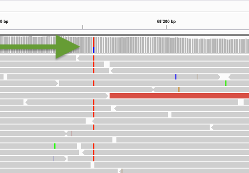
Suggestion
A clear heterozygous site as sufficient forward and reverse reads support it.
Suggestion
Could be an indel but it is not well supported.
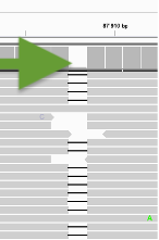
Suggestion
Not a clear heterozygous site as the alternative allele of the SNP is not well supported.

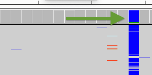
Suggestion
Not clear the heterozygous sites are supported by only 1 read.
SNP calling
Login to our server.
ssh guest?@gdc-vserver.ethz.ch
Let's go to the mapping folder.
cd mapping
We will continue working on the Chitidia dataset and will do now a variant calling.
First, we need to generate a list with all bam files as we like to do a joint calling.
ls -1 *_nodup.bam > bam.lst
Let's now run bcftools using the default settings and the multi-allele model. Indels we remove and have the depth and the allelic depth flag activated.
bcftools mpileup -f Ref_C_bombi.fasta --skip-indels -b bam.lst -a 'FORMAT/AD,FORMAT/DP' | bcftools call -mv -Oz -o raw.vcf.gz
❖ Challenge #2 How many SNPs are in total?
Suggestion #2
We count the number of lines but exclude lines starting with #.
zcat raw.vcf.gz| grep -v '^#' | wc -l
❖ Challenge #3 Have a look at the SNP table. Try to understand the vcf file format. What are the genotypes of the 4 samples on scaffold3_8_ref0000002_ref0000084 and position 100.
Suggestions #3
scaffold3_8_ref0000002_ref0000084    100
 ERR3418932  AA
 ERR3418936 AA
 ERR3418937  AT
 ERR3418961 NA
SNP filtering
In order to filter false positive SNPs we are going to apply some hard filters. The filters presented here is only a subset. In the RAD section you find more.
First we need to load the snp conda module that we can use vcftools.
conda activate /usr/bin/condaenv/snps
Set sites with less than 3 reads to NA and keep only sites with a minimum mapping quality of 30.
vcftools --gzvcf raw.vcf.gz --minQ 30 --minDP 3 --recode --recode-INFO-all --stdout | gzip -c > raw_Q30_minDP3.vcf.gz
Lets remove low quality sites using the integrated filtering script.
bcftools view raw_Q30_minDP3.vcf.gz | vcfutils.pl varFilter - | gzip -c > raw_Q30_minDP3_Qual.vcf.gz
As we have seen that the coverage varies a lot, we will remove sites with low or extremly high coverge.
Let's calculate the mean coverage across the sites.
vcftools --gzvcf raw_Q30_minDP3_Qual.vcf.gz --site-depth
Then we need to divide the values by the number of indiviudals 4 in our case and plot the vaues.
cut -f3 out.ldepth | awk '{print $1/4}' > meandepthpersite

gnuplot << \EOF
set terminal dumb size 200, 30
set autoscale
set xrange [20:120]
unset label
set title "Histogram of mean depth per site"
set ylabel "Number of Occurrences"
set xlabel "Mean Depth"
binwidth=1
bin(x,width)=width*floor(x/width) + binwidth/2.0
set xtics 5
plot 'meandepthpersite' using (bin($1,binwidth)):(1.0) smooth freq with boxes
pause -1
EOF
Let's set mean min-meanDP to 55 and max-meanDP to 90.
vcftools --gzvcf raw_Q30_minDP3_Qual.vcf.gz --min-meanDP 55 --max-meanDP 90 --recode --recode-INFO-all --stdout | gzip -c > raw_Q30_minDP3_Qual_meanDP55_maxDP90.vcf.gz
❖ Challenge #4 How many variants are you retaining?
Remove sites with more than 5% missing sites.
vcftools --gzvcf raw_Q30_minDP3_Qual_meanDP55_maxDP90.vcf.gz --max-missing 0.95 --recode --recode-INFO-all --stdout | gzip -c > raw_Q30_minDP3_Qual_meanDP55_maxDP90_NA95.vcf.gz
❖ Challenge #5 How many variants do you retain?
Finally, we only keep bi-allelic sites.
vcftools --gzvcf raw_Q30_minDP3_Qual_meanDP55_maxDP90_NA95.vcf.gz --min-alleles 2 --max-alleles 2 --recode --recode-INFO-all --stdout | gzip -c > raw_Q30_minDP3_Qual_meanDP55_maxDP90_NA95_SNPs.vcf.gz
❖ Challenge #6 What is the final numbers of SNPs in your table?
Manual inspection of the SNPs
Let's go back to the IGV view, load open again the bam files and add this time the vcf files on top.
❖ Challenge #7 Can you verify some of the SNPs manually? Do you see differences between the filter and the raw vcf? Make some print screens.
Increasing sample size
In many cases having replicates helps you to understand a biological pattern. We going to use a vcf file including more samples.
Let's download some more files.
curl -O https://www.gdc-docs.ethz.ch/GeneticDiversityAnalysis/GDA/data/more_SNP.tar.gz
tar xvzf more_SNP.tar.gz && rm more_SNP.tar.gz
cd more_SNP
The information about the samples are provided in popmap.
| Sample | Species |
|---|---|
| ERR3418932 | CB |
| ERR3418936 | CB |
| ERR3418937 | CB |
| ERR3418955 | CB |
| ERR3418956 | CB |
| ERR3418957 | CB |
| ERR3418958 | CB |
| ERR3418959 | CB |
| ERR3418960 | CB |
| ERR3418961 | CEX |
| ERR3418963 | CEX |
To get a first impression of the global picture we are performing a Principal Component Analysis (PCA). We are going to execute the R script directly in the terminal (PCA_vcf.R). To run an R-script on the command-line in order to generate a PCA and produce a pdf you just need to call the script with your filtered vcf file and the population information. The file popmap contains some basic information about the samples in this dataset.
Rscript --vanilla PCA_vcf.R more_samples_raw.vcf.gz popmap
❖ Challenge #9 What do you think about the PCA? How representative is this plot? Do we need to exclude samples? Missing sites could be a problem in PCAs. Let's output the missing sites per individual.
vcftools --gzvcf more_samples_raw.vcf.gz --missing-indv
❖ Challenge #10 Do we need to exclude sample(s)? With the following command you can generate a list with samples to exclude.
echo "XXX" >  miss_Ind.txt
echo "YYY" >>  miss_Ind.txt
vcftools --gzvcf more_samples_raw.vcf.gz --remove miss_Ind.txt --recode --recode-INFO-all --stdout | gzip -c > more_samples_raw_reduced.vcf.gz
Let's filter the reduced dataset and re-plot the PCA. Any comments on the PCA?