Multicollinearity

Multicollinearity occurs when predictor variables are highly correlated with each other. It makes individual variable effects difficult to estimate reliably: coefficients become unstable, standard errors inflate, and interpretation becomes ambiguous.

It is important to distinguish between two situations:

Inference (which variables matter, what drives the pattern): multicollinearity is a serious problem
Prediction (how well can I predict the outcome): multicollinearity is much less of a concern

Common examples in biology include body weight and body length, genes in the same pathway, temperature and humidity, or multiple measures of the same trait such as leaf length and leaf area.

Detection

Correlation matrix

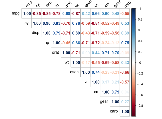
A natural first step after computing correlations. Pairwise values above roughly |r| = 0.8 are worth investigating, but pairwise correlations alone cannot detect all forms of multicollinearity.

library(corrplot)

corrplot(cor(mtcars),
         method = "number",
         type = "upper",
         tl.col = "black",
         tl.srt = 45)

Correlation matrix of the mtcars dataset. Values above |r| = 0.8 indicate potential multicollinearity.

Variance Inflation Factor (VIF)

VIF is the standard diagnostic for regression models. It quantifies how much the variance of a coefficient is inflated due to collinearity with other predictors:

library(car)

model <- lm(mpg ~ cyl + disp + hp + wt, data = mtcars)
round(car::vif(model), 2)
#>  cyl   disp     hp     wt
#> 6.74  10.37   3.41   4.85

disp has a VIF well above 10, indicating severe collinearity, and cyl is also elevated at 6.74. This is consistent with both variables capturing overlapping information about engine size, and their individual effects on mpg cannot be reliably separated from one another. hp and wt show less collinearity with the other predictors, although the VIF values should still be interpreted in context.

VIF	Rough interpretation
1	No inflation
1 to 5	Usually modest
5 to 10	Potentially concerning
> 10	Often considered severe

These are rules of thumb, not universal thresholds. Whether collinearity is problematic depends on the research question, sample size, and model.

Solutions

Which solution fits depends on your goal:

graph TD
    A[Multicollinearity detected] --> B{Primary goal?}
    B -->|Interpretation| C{How many variables?}
    B -->|Prediction| D[PCA or Ridge regression]
    C -->|Few| E[Remove or combine variables]
    C -->|Many| F[Lasso regression]

Remove one variable from a correlated pair. Keep the one with the clearer biological interpretation. In the mtcars example, cyl and disp both measure engine size, so keeping disp alone substantially reduces the collinearity, although its VIF remains elevated.

model2 <- lm(mpg ~ disp + hp + wt, data = mtcars)
round(car::vif(model2), 2)
#>  disp    hp    wt
#>  7.32  2.74  4.84

Combine variables into a single composite. This works best when two predictors measure the same underlying quantity. Combining leaf length and leaf width can provide an approximate measure of leaf area, replacing two correlated predictors with one ecologically meaningful variable. The composite should always have a clear interpretation.

PCA replaces a set of correlated variables with uncorrelated principal components. This can be a useful solution when many correlated variables are involved, but the components are linear combinations of the originals and can be harder to interpret biologically. In the mtcars example, the first component typically captures a general engine size gradient explaining over 80% of the variance among the four predictors:

pca <- prcomp(mtcars[, c("cyl", "disp", "hp", "wt")], scale. = TRUE)
summary(pca)  # PC1 usually explains > 80% here

model <- lm(mpg ~ pca$x[, 1] + pca$x[, 2], data = mtcars)
# Coefficients now refer to components, not the original variables

Regularised regression stabilises estimates by penalising large coefficients without removing variables beforehand. Ridge shrinks all coefficients toward zero but retains every predictor, which makes it useful for prediction. Lasso sets some coefficients exactly to zero, effectively selecting a subset of variables and making results more interpretable:

library(glmnet)

X <- as.matrix(mtcars[, c("cyl", "disp", "hp", "wt")])
y <- mtcars$mpg

set.seed(123)
cv_ridge <- cv.glmnet(X, y, alpha = 0)  # Ridge: keeps all variables
cv_lasso <- cv.glmnet(X, y, alpha = 1)  # Lasso: excludes some variables

coef(cv_lasso, s = "lambda.min")
#             lambda.min
# (Intercept)  38.39955859
# cyl          -0.93640004
# disp          .
# hp           -0.01718336
# wt           -3.10649607
# Coefficients set to exactly zero are excluded from the model

Here, lasso drops disp entirely while keeping cyl, hp, and wt, consistent with disp and cyl capturing overlapping information about engine size, as noted above. The exact coefficients (and which variable gets dropped) can shift slightly with different random cross-validation folds, so treat this as an illustration of the general pattern rather than a fixed result.

Strategy	Variables kept	Interpretability	Best for
Remove	Fewer	High	Few correlated pairs
Combine	Fewer	Medium	Biologically meaningful composites
PCA	Components	Lower	Many correlated variables
Ridge	All	Medium	Prediction with correlated predictors
Lasso	Some	High	Variable selection and prediction

Exercise

Using the iris dataset, build a model predicting Sepal.Length from the other three numeric variables. Detect multicollinearity and apply an appropriate solution.

Solution

library(car)

model <- lm(Sepal.Length ~ Sepal.Width + Petal.Length + Petal.Width,
            data = iris)
round(car::vif(model), 2)
#> Sepal.Width  Petal.Length  Petal.Width
#>        1.27         15.10        14.23

# Petal.Length and Petal.Width are severely collinear
# Option 1: remove one of the redundant predictors
model2 <- lm(Sepal.Length ~ Sepal.Width + Petal.Length, data = iris)
vif(model2)  # Both now near 1.3

# Option 2: replace both with a PC
pca <- prcomp(iris[, 3:4], scale. = TRUE)
model3 <- lm(Sepal.Length ~ Sepal.Width + pca$x[, 1], data = iris)