OTU/Count Table (Matrix)

What a count table looks like, why it behaves the way it does statistically, and how to normalise it responsibly.

This is arguably the single most important file you get from us. Almost everything downstream, diversity metrics, ordinations, statistical tests, community comparisons, is computed from this one table. Understanding its structure and quirks matters more than knowing any individual command in your analysis script. If you become comfortable reading this table, you'll understand most of what happens in the rest of your analysis.

Schematic Layout

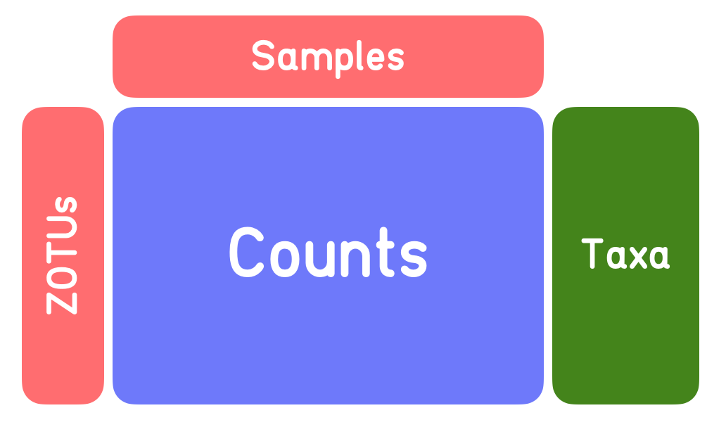
	Sample A	Sample B	Sample C	Mock	Negative	Taxa
ZOTU1	5000	24	2	0	3	KCOFGS
ZOTU2	1202	546	34	734	0	KCOFGS
ZOTU3	560	899	124	0	0	KCOFGS
ZOTU4	12	356	5461	0	0	KCOFGS
ZOTU5	0	0	65	0	0	KCOFGS
ZOTU6	0	5	0	0	1	KCOFGS
ZOTU7	0	34	0	0	2	KCOFGS
ZOTU8	0	0	453	1432	0	KCOFGS
ZOTU9	1	0	0	243	12	KCOFGS
ZOTU10	0	0	0	546	0	KCOFGS
...

Each row is a cluster, an OTU or zOTU, and each column is a sample. A cell is the number of reads assigned to that cluster in that sample. The numbering itself carries information: OTUs and zOTUs are numbered by descending total abundance, so ZOTU1 is your single most abundant cluster across the whole dataset, ZOTU2 the second most abundant, and so on. A low number is a quick, rough proxy for "this one showed up a lot," worth keeping in mind before you go looking up what ZOTU847 actually is. This also means the two properties are directly linked: because OTUs are numbered by descending abundance, the number of samples with a zero for a given OTU tends to climb as the OTU number climbs. A handful of low-numbered OTUs are usually present, in some amount, across most of your samples, while the long tail of high-numbered OTUs are often detected in only one or two samples, or even just once in your entire dataset, and are zero everywhere else. That long tail is normal for amplicon data and is part of why the table is so sparse overall, not a sign that something went wrong with those particular clusters.

Check This Against the Example Table

The illustrative numbers in the table above don't actually follow this rule: ZOTU4's row sums to 5829 reads, higher than ZOTU1's 5029, yet ZOTU1 is listed first. That's fine if this table was only ever meant to illustrate structure and sparsity rather than real abundance ranking, but worth fixing (or reordering the example rows) before publishing, so an attentive reader who adds up the numbers doesn't end up doubting the rule you just stated.

This orientation, features (OTUs/zOTUs) in rows and samples in columns, is common in bioinformatics generally, though not universal: some software, including certain phyloseq import paths, expects the transpose, so if you get an orientation error on import, that's usually the first thing to check. The Taxa column carries the taxonomic call for the row, at whatever ranks were resolved (see Data Prep Short-Reads (PE), Step F for how those assignments are made and why they should be treated as hypotheses, not certainties).

Mock and Negative Aren't Regular Samples

Two of the columns above aren't experimental samples at all, and you'll usually find equivalents in your own table.

A Mock community is a sample of known composition, included specifically to validate the pipeline. Because you know in advance which taxa should be there and roughly in what proportion, it lets you sanity-check clustering, taxonomic assignment, and cross-talk correction against ground truth, rather than trusting the pipeline blindly.

A Negative control should contain little to no biological material, so it should come back with very few reads. Non-zero counts here point to contamination or index cross-talk (see the Data Prep Output page's note on UNCROSS) rather than to real biology, and are exactly the kind of higher-than-average data loss flagged in the Data Prep Short-Reads (PE) page's caution about negative controls skewing summary statistics if included in project-wide averages.

Keep both out of your biological comparisons, but keep an eye on them: they're your best evidence that the pipeline behaved correctly on your specific run.

About the Taxa Column

The KCOFGS shorthand above stands for Kingdom, Class, Order, Family, Genus, Species, six ranks read left to right. If that looks like it's missing a rank to you too, you're not wrong: the conventional Linnaean order used in most taxonomy databases is Kingdom, Phylum, Class, Order, Family, Genus, Species (KPCOFGS). We're flagging this rather than silently fixing it, since we don't want to guess whether Phylum was deliberately left out for a specific marker or reference, or whether this is simply a long-standing typo in the schematic. Worth confirming before this goes live.

Table Characteristics

Raw read counts. Every value is a non-negative integer, a direct count of reads, not yet a proportion, percentage, or normalised abundance. Whether and how to convert these counts into something comparable across samples is exactly the subject of the normalisation section below.
Many zeros. Most taxa are absent from most samples, which is expected both biologically (real community turnover between samples) and technically (a taxon can be genuinely present at low abundance yet simply not get picked up in a given sample's read depth by chance). Telling these two kinds of zero apart is often impossible from the count table alone. Tables like this are often described as sparse, since most cells contain zero, a term you'll run into constantly once you start reading about microbiome statistics.
Differences in sequencing depth. Total reads per sample vary, sometimes substantially, for reasons that have nothing to do with biology: pooling variation, index balance, and general run-to-run noise. This is a sequencing artefact, and comparing raw counts directly across samples with different depths will make some samples look more or less diverse than they really are, purely as an artefact of how much was sequenced.
Differences in library composition. This one is biological rather than technical, but no less important: if one taxon genuinely dominates a sample, it mechanically suppresses the apparent counts of every other taxon in that sample, since they're all competing for a fixed number of sequencing reads. A taxon's true abundance can stay constant while its apparent count drops, simply because something else in the same sample became more abundant.

Table Summary

cat e_OTU/*_ZOTU_Count.summary

See the Data Prep Output page for what this report contains: total reads, number of samples, number of (z)OTUs, and a detailed count breakdown.

Data Characteristics

These are the formal statistical properties behind the table characteristics above, and the reason count tables need careful handling rather than off-the-shelf statistical methods designed for other kinds of data.

Compositional. The counts in a sample are constrained by that sample's fixed sequencing depth, so they represent relative proportions of a whole, not independent absolute abundances. This is the formal version of the "library composition" point above, and it's the single biggest reason naive statistics on raw counts go wrong: a change in one taxon's proportion necessarily changes every other taxon's apparent proportion too, even without any real biological change in the others. Imagine one species blooms dramatically in a sample. Even if every other species in that sample stays at exactly the same absolute abundance, their read counts will usually go down anyway, because the sequencing run now spends a larger fraction of its fixed number of reads on the blooming species, leaving fewer reads for everything else:
```
True abundance (before)          Read counts, fixed depth of 1000
  A: 10                            A: 333
  B: 10                            B: 333
  C: 10                            C: 334

True abundance (after A blooms)  Read counts, same fixed depth of 1000
  A: 20  (doubled)                 A: 500
  B: 10  (unchanged)               B: 250  ← looks like it dropped
  C: 10  (unchanged)               C: 250  ← looks like it dropped
```
B and C didn't change at all, but their read counts drop simply because A is now taking up a bigger share of a fixed sequencing budget.
Zero-inflated / sparse. There are more zeros than standard count distributions expect, which complicates both modelling and normalisation, particularly for any method that involves a log transformation, since the log of zero is undefined and forces a decision about how to handle it (a pseudocount, a zero-replacement strategy, or a method designed to tolerate zeros directly).
Overdispersed. A simple Poisson model assumes the variance of a count equals its mean, so if a taxon averages 100 reads across replicate samples, Poisson expects a standard deviation around 10. Real amplicon data blows way past that: the same taxon might show a standard deviation of 40 or 50 across true replicates, not because anything went wrong, but because PCR amplification bias, uneven cell lysis, and patchy micro-scale distribution of organisms all add variability on top of ordinary sampling noise. A model that assumes Poisson variance will report tighter confidence intervals and smaller p-values than the data actually supports, making differences look more significant than they are. Models built for overdispersed count data (e.g. the negative binomial models used in tools like DESeq2 or edgeR) generally fit better, since they allow variance to exceed the mean instead of assuming they're equal.
High dimensional. Datasets typically have far more taxa (features) than samples (data points), which complicates statistical testing, demands correction for multiple comparisons, and makes many multivariate models prone to overfitting if applied naively.
Underdetermined. A more theoretical, but related, consequence of high dimensionality: with more OTUs than samples, some matrix operations that certain multivariate methods rely on (e.g. inverting a covariance matrix) aren't well-defined without additional constraints or dimension reduction. You're unlikely to run into this directly unless you're implementing a method yourself rather than using an existing package, but it's part of why some multivariate tools need extra care with this kind of data.

Count "Normalisation" Approaches

There are several approaches to correcting for one or more of the data structure difficulties above. None of them fixes everything at once, and which one is appropriate depends on your downstream analysis, which is why we put "normalization" in quotes: it's less a single solved procedure and more a set of trade-offs to choose between deliberately.

Rarefying. Subsample every sample down to the same fixed number of reads (typically the count of your shallowest acceptable sample), discarding the rest. This directly equalises sequencing depth, at the cost of throwing away real data from your deeper samples.
Total count scaling / proportions. Divide each count by the sample's total, converting counts into proportions. Simple and keeps all your data, but does nothing to address compositionality, and can behave poorly with the very uneven, zero-heavy distributions typical of amplicon data.
Scaling with size factors (effective library sizes). Methods borrowed from RNA-seq (e.g. DESeq2, edgeR) estimate a per-sample scaling factor from the overall count distribution rather than just the raw total, aiming to be less sensitive to a handful of very abundant taxa dominating the total count.
Data transformation. Log-ratio transformations (e.g. centered log-ratio, CLR) explicitly treat the data as compositional and transform it into a space where standard statistical methods behave better, generally requiring a strategy for handling zeros first.

There is no universally correct choice here. The right approach depends on what your downstream analysis is actually asking, whether that's alpha diversity, beta diversity and ordination, differential abundance testing, or something else, since different methods were developed and validated for different questions.

This Is a Genuinely Contested Question

Which of these approaches is "best" is an active, sometimes heated methodological debate in microbial ecology, not a settled matter. The literature below leans toward rarefaction, which has data behind it, but a widely cited earlier paper argued the opposite position: McMurdie and Holmes (2014), "Waste not, want not: why rarefying microbiome data is inadmissible," PLoS Computational Biology 10:e1003531. If you're choosing a normalisation strategy for a specific analysis, it's worth being aware that reviewers may hold either position strongly, and being prepared to justify your choice rather than assuming it's uncontroversial. Ask us if you'd like help thinking through which approach fits your specific downstream analysis.

Literature

Schloss (2023) Rarefaction is currently the best approach to control for uneven sequencing effort in amplicon sequence analyses. bioRxiv 2023.06.23.546313; published as Schloss (2024) mSphere e0035523; doi.org/10.1128/msphere.00354-23
McMurdie and Holmes (2014) Waste not, want not: why rarefying microbiome data is inadmissible. PLoS Computational Biology 10:e1003531.