Overview Workflows
How Illumina, PacBio and AVITI data differ, and how to pick a clustering strategy for each.
There are different ways of generating metabarcode (AmpSeq) data, and these change over time. It is important to understand exactly how your samples were processed, which library preparation was used, and how the data was sequenced. The better you understand these steps, the better the downstream processing will be.
Which Workflow Applies to Me?
| Your data | Workflow |
|---|---|
| Illumina paired-end (MiSeq, MiSeq i100) | Merge forward and reverse reads, then cluster |
| AVITI paired-end | Same as Illumina: merge, then cluster |
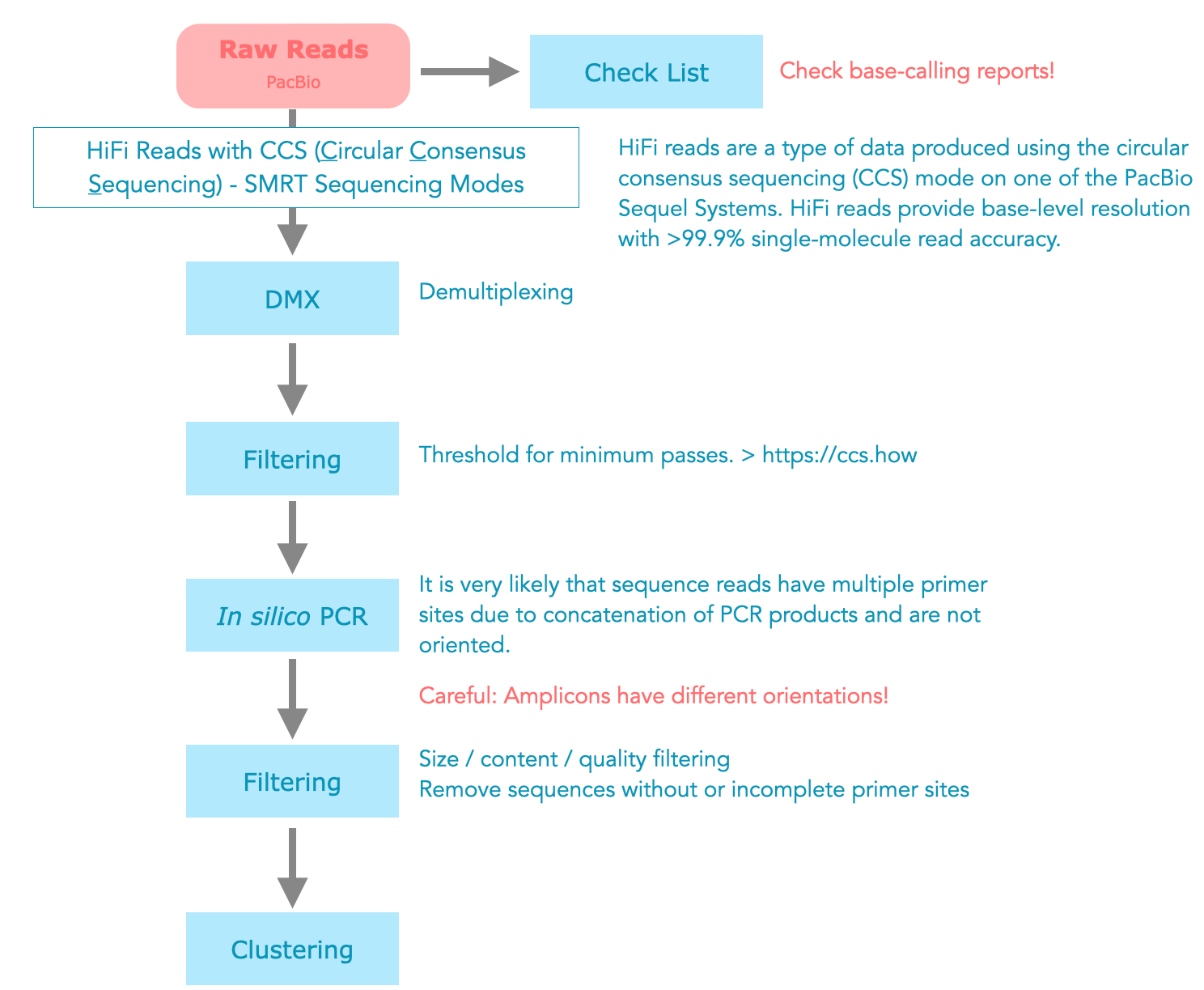
| PacBio CCS / HiFi | No merging needed, orient and clean, then cluster |
| PacBio Kinnex | Deconcatenate the array first, then follow the PacBio CCS workflow |
| Oxford Nanopore (ONT) | We do not currently recommend ONT for amplicon sequencing, see below |
If you are not sure which of these applies to your project, the platform sections below explain what to look for in your raw data.
The Pipeline, in Brief
Regardless of platform, every amplicon project moves through the same broad stages:
Raw reads → Cleaning (quality filtering, primer trimming, and for paired-end data, merging) → Clustering into OTUs or zOTUs → Taxonomic assignment
The details of each stage depend on your sequencing platform, your marker gene, and your project's goals, which is what the rest of this page walks through.
A note on marker genes. Which marker you sequence depends on what you're studying. Common choices include 16S rRNA for bacteria and archaea, ITS for fungi, 18S rRNA for eukaryotes more broadly, COI for animals, and rbcL for plants. If you're not sure which marker your project uses, that's worth confirming before you get too far into processing, since it affects primer trimming, expected amplicon length, and which reference database applies.
Illumina
Most amplicon sequencing projects we process at the GDC are paired-end MiSeq based data sets with dual-indexing. The index (also known as barcode) is read separately, and demultiplexing (index sorting) of the sequence reads is done by, for example, the MiSeq Control Software (MCS).
We currently run two machines: an older MiSeq and the newer MiSeq i100.
MiSeq vs. MiSeq i100
The i100 supports longer paired-end reads than the older MiSeq, which pushes the maximum usable amplicon size well beyond what we could cover before, opening the door to full-length 16S and other longer markers on a benchtop Illumina run where previously you would have needed PacBio for that range.
Read quality is also noticeably better, and the usual quality drop-off towards the end of a read, especially on the reverse read, is much less pronounced. In our experience the gap between forward and reverse read quality has become almost invisible.
On top of that, the i100 simply gives you more data for the same cost, so deeper sequencing or larger sample numbers per run are more affordable than they used to be.
Exact cycle counts and read lengths depend on the kit and change as Illumina updates its offering, so we won't quote figures here. Ask us if you want current numbers for your specific project.
A single run should give you files per sample. In most cases that means just two:
- Forward read: SampleA_R1.fq.gz
- Reverse read: SampleA_R2.fq.gz
This is the default you should expect, from us and from most sequencing facilities generally: the instrument demultiplexes reads per sample using the index reads internally, and only R1 and R2 get exported, since the index reads have already done their job by that point.
Raw Index Reads: An Older-MiSeq Option, Not the i100
On our older MiSeq, we can optionally also export the raw index reads themselves, giving you 4 files per sample instead of 2 (adding SampleA_I1.fq.gz and SampleA_I2.fq.gz). This is useful in specific troubleshooting situations, verifying demultiplexing, checking for index hopping, or handling a combinatorial indexing scheme MCS doesn't demultiplex natively, and costs nothing extra, so it's worth asking for if you think you might need it. But it isn't something most facilities offer as standard, and it isn't available at all on the MiSeq i100: there's no equivalent export option there, so i100 runs only ever give you the 2-file version. As we move more projects to the i100, expect this option to become less relevant going forward, not more.
PacBio CCS Reads
More and more projects use PacBio HiFi reads (CCS). Each sample typically comes with several raw files, but only one matters for amplicon sequencing: a BAM file containing the CCS reads themselves. These reads are produced by sequencing the same circular DNA molecule multiple times and combining the passes into a single, highly accurate consensus sequence, hence Circular Consensus Sequencing (CCS), also marketed as HiFi.
Files are usually named:
<sample_name>*ccs*.bam or <sample_name>*hifi*.bam
PacBio Sequence Orientation
PacBio sequences are normally not oriented and need to be aligned. There are also composite sequences with multiple primer sites. These must either be cleaned up or removed.
Increasingly, amplicon libraries are prepared and sequenced using PacBio's Kinnex chemistry, which concatenates several amplicons into a single array per ZMW well before sequencing. These arrays need to be segmented (deconcatenated) into individual amplicon reads before anything else can happen, a step the standard CCS workflow above does not cover. If your data came from a Kinnex library, let us know before you start demultiplexing, since it changes the first step of the pipeline.
How the data can be delivered. Depending on how your sequencing was set up, you may receive your data in different states:
- A single BAM file per run, still concatenated (if Kinnex was used) and not yet demultiplexed by sample.
- Deconcatenated and demultiplexed FASTQ files, one pair (or set) per sample, already split out for you.
Our Preference: Do the Demultiplexing Ourselves
Even when demultiplexed FASTQ files are offered, we prefer to start from the undemultiplexed BAM file and do this step ourselves. This gives us a direct view of run performance that you lose once the data has already been split, including reads that carried a barcode combination that was not actually used in the sample sheet. A high proportion of such reads often points to barcode misassignment, cross-contamination, or a mistake in the sample sheet itself, and this is much easier to catch before demultiplexing than after. If you already have demultiplexed FASTQ files, that is fine to send us too, but where possible, please also keep the original BAM file available in case we need to revisit the demultiplexing.
Deconcatenation Is Not Always Straightforward
We can also perform the deconcatenation step for Kinnex data ourselves. For the standard 16S-Kinnex kit this is well established and usually runs smoothly. For other marker genes or custom Kinnex array designs, deconcatenation is trickier, since the segmentation depends on knowing the exact array structure and adapter layout used, which is not always well documented outside the standard kits. If you are using a non-standard Kinnex setup, talk to us early so we can check whether the standard tools apply or whether extra groundwork is needed first.
Element Biosciences (AVITI)
Another option has recently entered the market. EB's AVITI is a promising alternative to Illumina, and we have been gathering experience with it.
So far we like what we see. Read quality is good, and the number of reads per run is high, in the range of 600 to 700 million in our hands. The main limitation is read length: AVITI currently tops out at 2 x 300 bp, so unlike the MiSeq i100, it is not an option for amplicons that need longer paired-end reads to cover full-length markers.
PCR-Free Accuracy
AVITI uses Rolling Circle Amplification (RCA) for clonal amplification instead of PCR, combined with Sequencing by Binding (SBB) rather than the sequencing-by-synthesis (SBS) chemistry used by Illumina. Together these significantly reduce duplication rates and index hopping compared to what we typically see on patterned Illumina flow cells.
We are continuing to build experience with AVITI and will expand this section as our own data accumulates.
Oxford Nanopore (ONT)
ONT is tempting on paper: long reads, low upfront cost, and a portable instrument. It has genuine strengths for other applications, including long-read assembly, structural variant detection, and real-time monitoring in the field. For amplicon sequencing specifically, though, we do not currently recommend it.
The core issue is error rate. ONT's raw read accuracy has improved substantially over the last few chemistry generations, and recent kits and duplex basecalling can approach the accuracy of short-read platforms under favourable conditions. But amplicon sequencing is exactly the setting where that residual error matters most: an amplicon dataset is built from many near-identical short sequences, and clustering or denoising needs to reliably tell a genuine single-nucleotide biological difference apart from a sequencing error. Illumina, AVITI, and PacBio CCS reads all give that distinction a solid footing. With ONT, the raw error rate still sits close to, or above, the level of real biological variation you are often trying to detect, which makes robust OTU or zOTU calling considerably harder, particularly for markers where strain- or species-level resolution matters.
This is a fast-moving area, and we will revisit this recommendation as ONT chemistry and metabarcoding-specific tools continue to improve. If you are considering ONT for a project regardless, for example because portability or field use is a hard requirement, talk to us first so we can flag what to expect and what the current workarounds cost you in resolution.
Workflow Overview
Illumina, PacBio, and AVITI data differ in more than just read length, so processing steps need to be adapted to the sequencing platform. Even within the same technology, it is worth adapting the processing steps to the specific structure of your data, for example how much your paired-end reads overlap, or whether your samples are unusually low or high in diversity.
AVITI's paired short-read output is processed the same way as Illumina paired-end data (Figure 1). PacBio CCS/HiFi reads follow a different path (Figure 2), since each read already covers the full amplicon on its own rather than arriving as a forward/reverse pair that needs merging.
This cuts both ways. Skipping the merging step removes a possible source of error: merging can go wrong wherever primers, overlap length, or read quality make it ambiguous how forward and reverse reads should be stitched together, and misjudged overlaps can introduce artefacts of their own. But merging is not only a source of error, it is also a correction step. Where forward and reverse reads overlap and disagree at a position, the base with the better quality score usually wins, effectively letting the two reads check each other. PacBio CCS reads do not have an equivalent second read to cross-check against; their accuracy instead comes entirely from the multiple internal passes around the same circular molecule that produce the consensus read in the first place. Both strategies work well, they just correct errors at different stages and by different means.
Figure 1: Possible workflow scenarios for paired-end (Illumina and AVITI) data.

Figure 2: Possible workflow for PacBio CCS data.
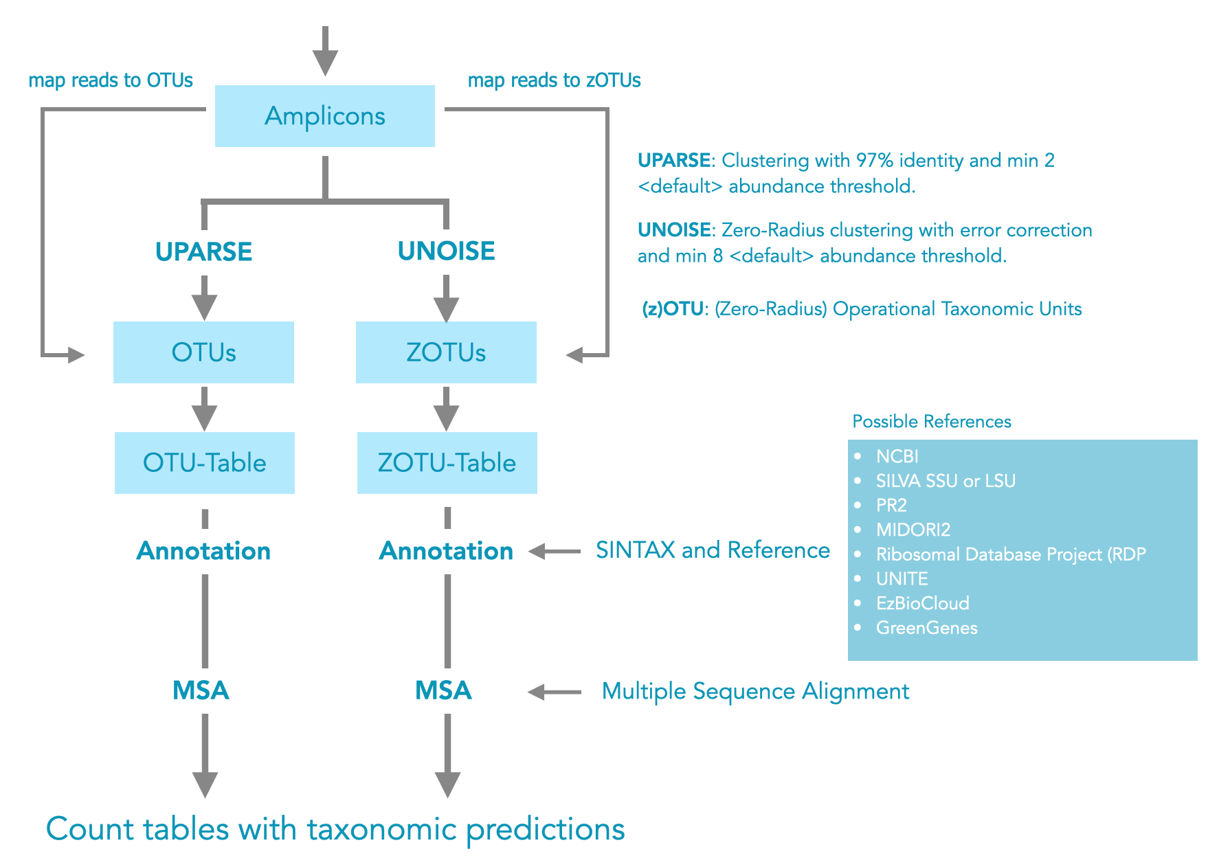
Once the data is cleaned (quality filtered, primer-trimmed, and for paired-end data merged into a single amplicon sequence), clustering begins. Two approaches are commonly used to group the cleaned amplicons into biologically meaningful units.
OTU clustering (UPARSE). Sequences are grouped into clusters within a 3% radius (97% identity). Clusters supported by only a single sequence (singletons) are usually discarded, since these are hard to tell apart from noise. UPARSE does a good job at this, but the algorithm is greedy: there are several equally valid ways to draw the cluster boundaries, not one single best solution, so repeating the clustering step on the same input can shift the result very slightly.
zOTU denoising (UNOISE, comparable to ASVs). Rather than clustering by a fixed similarity radius, UNOISE tries to correct sequencing errors and recover the true underlying biological sequences at single-nucleotide resolution. Low-abundance sequences that differ from a much more abundant sequence by only one or a few bases are treated as likely errors of that sequence and folded into it. Sequences that remain distinct after this correction, and clear a minimum abundance threshold, become zero-radius OTUs (zOTUs). This is conceptually similar to the Amplicon Sequence Variant (ASV) approach used by tools such as DADA2.
Both approaches remove chimeras by default. Neither is simply "more correct" than the other: OTU clustering is more forgiving of residual sequencing error and gives a coarser, more stable grouping, while zOTUs preserve fine-scale sequence variation but are more sensitive to how the denoising parameters are set. Which one fits your project depends on your question and your marker gene.
| OTUs (UPARSE) | zOTUs (UNOISE) | |
|---|---|---|
| Method | 97% similarity clustering | Error-correction / denoising |
| Resolution | Coarser | Single-nucleotide |
| Tolerance to residual noise | More forgiving | More sensitive to parameters |
| Comparable to | Traditional OTU picking | ASVs (e.g. DADA2) |
| Good fit for | Broad community comparisons, robustness across runs | Strain-level differences, fine-scale variation |
Figure 3: Sequence clustering.
Recommended Workflows at a Glance
Not sure where to start? Here's what we typically recommend, though your specific project may call for something different, so treat this as a starting point rather than a rule.
| Data | Recommended starting point |
|---|---|
| MiSeq / MiSeq i100 paired-end | Merge, then UNOISE (zOTUs) for fine-scale resolution, or UPARSE for broad community comparisons |
| AVITI paired-end | Same as Illumina |
| PacBio CCS / HiFi | Orient, trim, then UNOISE (zOTUs) |
| PacBio Kinnex | Deconcatenate first, then follow the PacBio CCS route above |
A Note on Preference
USEARCH is now open source, as of version 12. Earlier versions (5 through 11) were free to use for non-commercial purposes but closed-source, with a paid licence required for commercial or for-profit use. VSEARCH remains a solid open-source alternative that reimplements most of the same algorithms and has been fully open throughout.
We prefer USEARCH and VSEARCH over integrated pipelines such as QIIME2 or mothur, not because they are objectively better, but because they let us pick the right tool for each specific step rather than being handed one tool for everything. A pipeline that bundles trimming, merging, clustering, and taxonomy assignment into a single workflow is convenient, but each of those steps has its own decisions to make and its own failure modes, and a Swiss army knife approach trades precision at each step for convenience across all of them. We would rather run each step deliberately, inspect the intermediate output, and swap in a different tool if one step calls for it, than lose that visibility inside a monolithic pipeline.
Choosing a Reference Database
Taxonomic assignment is one of the trickier parts of the whole workflow. The result you get for a given OTU or zOTU depends on several factors at once: the classifier and its parameters, how the reference sequences were curated, and how well the reference actually covers your target group and marker region. A mismatch on any of these can quietly change your results without an obvious error message to warn you.
There are many excellent reference databases available, several actively maintained and offered in different formats, and the right one depends on your organism group and marker gene. Be careful about mixing references from different sources or curation standards within the same project, since inconsistent taxonomy or nomenclature between them can produce misleading results.
See Choosing a Reference Database for a full walkthrough of coverage, reliability, outgroups, and when it's worth building a custom reference.
Next Steps
Once you understand how your data was generated, head to Data Download to get your raw files, or jump straight to the workflow that matches your platform: Data Prep Short-Reads (PE), Data Prep Short-Reads (SE), or Data Prep Long-Reads.