Alpha Diversity Help

A quick summary to better understand alpha diveristy. To make this work, you need to download and import the dummy dataset described in chapter ”Phyloseq Help”.

## Subset Samples
d.A  <- subset_samples(d, GID == "A")
d.B  <- subset_samples(d, GID == "B")
d.AB <- subset_samples(d, GID == "A" | GID == "B")
d.C  <- subset_samples(d, GID == "C")

## There might be OTUs without counts after subsetting data
sum(taxa_sums(d.A) == 0)
sum(taxa_sums(d.B) == 0)
sum(taxa_sums(d.C) == 0)

## Remove the "zero" OTUs (if needed)
# d.A  <- prune_taxa(taxa_sums(d.A) > 0, d.A)

## OTU table overview
t(otu_table(d.A))

	OTU1	OTU2	OTU3	OTU4	OTU5	OTU6	OTU7	OTU8	OTU9	OTU10	OTU11	OTU12	OTU13	OTU14	OTU15
SA1	10	10	10	10	10	10	10	10	10	0	0	0	0	0	0
SA2	20	10	10	5	5	1	1	1	1	0	0	0	0	0	0
SA3	34	16	16	8	8	2	2	2	2	0	0	0	0	0	0
SA4	82	1	1	1	1	1	1	1	1	0	0	0	0	0	0
SA5	90	0	0	0	0	0	0	0	0	0	0	0	0	0	0

## Alpha-Diversity Table
alpha.diversity <- estimate_richness(d.A, measures = c("Observed", "Chao1", "Shannon", "InvSimpson"))
round(alpha.diversity, 3)

## A nice table
#DT::datatable(round(alpha.diversity, 3))

	Observed	Chao1	se.chao1	Shannon	InvSimpson
SA1	9	9	0.000	2.197	9.000
SA2	9	15	7.123	1.729	4.459
SA3	9	9	0.000	1.751	4.470
SA4	9	37	21.221	0.485	1.203
SA5	1	1	0.000	0.000	1.000

A table might be of limited use for larger data sets.

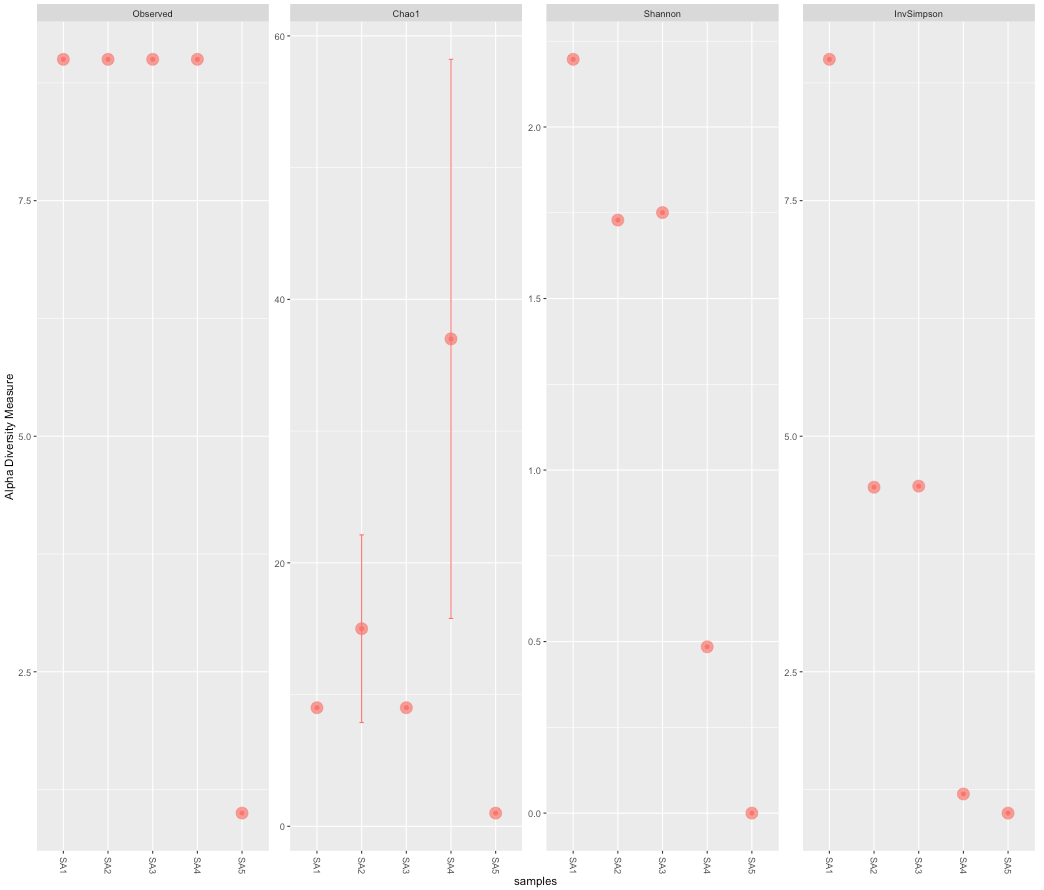
## Alpha-Diversity Plot
plot_richness(d.A, measures = c("Observed", "Chao1", "Shannon", "InvSimpson"))

## A "nicer" ggplot based plot
p <- plot_richness(d.A, color = "GID", measures = c("Observed", "Chao1", "Shannon", "InvSimpson"))
p + geom_point(size = 5, alpha = 0.7)

## Combined OTU and Diversity Tables
cbind(t(otu_table(d.A)), alpha.diversity)

It is easy to change the counts and play around with different values.

## Change Counts
otu_table(d.A)[,5]
otu_table(d.A)[,5] <- c(seq(90,10,-10))
otu_table(d.A)[,5]
otu_table(d.A)
estimate_richness(d.A, measures = c("Observed", "Chao1", "Shannon", "InvSimpson"))