Beta Diversity Help
A quick summary to better understand beta diveristy. To make this work, you need to download and import the dummy dataset described in chapter ”Phyloseq Help”.
Compositional Beat-Diversity
Help with Distance
distanceMethodList
betadiver(help = TRUE)
help(designdist) # designdist {vegan}
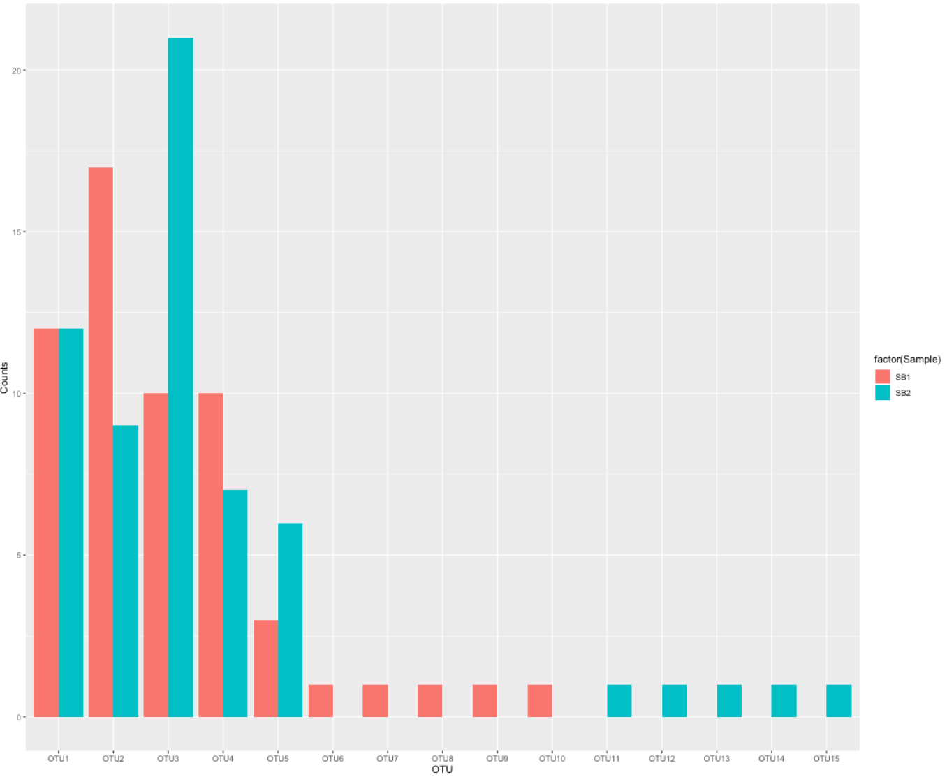
We use different OTU-abundance-distribution scenarios to better understand Beta-diversity indices.
### Example [A]: Frequent OTU overlap - rare ones are unique

## Explore data
t(otu_table(d.B))

## Wide-to-long format - ideal for ggplots!
x <- data.frame(otu_table(d.B))
x$OTU <- row.names(x)
x.new <- gather(x, Sample, Counts, SB1, SB2)

## Barplot

# Sample order - oneway or another
# position <- gtools::mixedsort(x$OTU)
position <- c("OTU1","OTU2","OTU3","OTU4","OTU5","OTU6","OTU7","OTU8","OTU9","OTU10","OTU11","OTU12","OTU13","OTU14","OTU15")

p <- ggplot(x.new, aes(x = factor(OTU, levels = position ), y = Counts, fill = factor(Sample))) +
  geom_bar(stat = "identity", position = "dodge") +
  xlab("OTU") + ylab("Counts")
p
We create a few more example cases and record the distances in a data frame:
## Create empty data frame
df <- setNames(data.frame(matrix(ncol = 4, nrow = 5)), c("Bray-Curtis (b)", "Jaccard (b)","Bray-Curtis (q)", "Jaccard (q)"))
row.names(df) <- c("Frequent-Overlap", "Frequent-Overlap(equal)", "Rare-Overlap", "Identical", "Different")

## Binary
dist.bc.b <- phyloseq::distance(d.B, method = "(A+B-2*J)/(A+B)")        ## "minimum" Bray-Curtis
dist.jc.b <- phyloseq::distance(d.B, method = "cc")                     ## Jaccard index of dissimilarity
dist.jc.b <- phyloseq::distance(d.B, method = "jaccard", binary = TRUE) ## vegdist jaccard

## Quantitative
dist.bc.q <- phyloseq::distance(d.B, method = "bray")                   ## Bray-Curtis
dist.jc.q <- phyloseq::distance(d.B, method = "jaccard")                ## Jaccard index of dissimilarity

df[1,1] <- dist.bc.b
df[1,2] <- dist.jc.b
df[1,3] <- dist.bc.q
df[1,4] <- dist.jc.q

### Example [B]: Frequent Overlap

## Change counts by hand
otu_table(d.B)[,1] <- c(20,10,10,5,5,1,1,1,1,1,0,0,0,0,0)
otu_table(d.B)[,2] <- c(20,10,10,5,5,0,0,0,0,0,1,1,1,1,1)
t(otu_table(d.B))

## Binary
dist.bc.b <- phyloseq::distance(d.B, method = "(A+B-2*J)/(A+B)") ## "minimum" Bray-Curtis
dist.jc.b <- phyloseq::distance(d.B, method = "cc")              ## Jaccard index of dissimilarity
## Quantitative
dist.bc.q <- phyloseq::distance(d.B, method = "bray")            ## Bray-Curtis
dist.jc.q <- phyloseq::distance(d.B, method = "jaccard")         ## Jaccard index of dissimilarity

df[2,1] <- dist.bc.b
df[2,2] <- dist.jc.b
df[2,3] <- dist.bc.q
df[2,4] <- dist.jc.q

### Example [C]: Rare Overlap

## Change counts by hand
otu_table(d.B)[,1] <- c(20,10,10,5,5,1,1,1,1,1,0,0,0,0,0)
otu_table(d.B)[,2] <- c(0,0,0,0,0,1,1,1,1,1,5,5,10,10,20)
t(otu_table(d.B))

## Binary
dist.bc.b <- phyloseq::distance(d.B, method = "(A+B-2*J)/(A+B)") ## "minimum" Bray-Curtis
dist.jc.b <- phyloseq::distance(d.B, method = "cc")              ## Jaccard index of dissimilarity
## Quantitative
dist.bc.q <- phyloseq::distance(d.B, method = "bray")            ## Bray-Curtis
dist.jc.q <- phyloseq::distance(d.B, method = "jaccard")         ## Jaccard index of dissimilarity

df[3,1] <- dist.bc.b
df[3,2] <- dist.jc.b
df[3,3] <- dist.bc.q
df[3,4] <- dist.jc.q

### Example [D]: Both identical

## Change counts by hand
otu_table(d.B)[,1] <- c(20,10,10,5,5,1,1,1,1,1,0,0,0,0,0)
otu_table(d.B)[,2] <- c(20,10,10,5,5,1,1,1,1,1,0,0,0,0,0)
t(otu_table(d.B))

## Binary
dist.bc.b <- phyloseq::distance(d.B, method = "(A+B-2*J)/(A+B)") ## "minimum" Bray-Curtis
dist.jc.b <- phyloseq::distance(d.B, method = "cc")              ## Jaccard index of dissimilarity
## Quantitative
dist.bc.q <- phyloseq::distance(d.B, method = "bray")            ## Bray-Curtis
dist.jc.q <- phyloseq::distance(d.B, method = "jaccard")         ## Jaccard index of dissimilarity

df[4,1] <- dist.bc.b
df[4,2] <- dist.jc.b
df[4,3] <- dist.bc.q
df[4,4] <- dist.jc.q

### Example [E]: Nothing in common

## Change counts by hand
otu_table(d.B)[,1] <- c(20,10,10,5,5,1,1,1,0,0,0,0,0,0,0)
otu_table(d.B)[,2] <- c(0,0,0,0,0,0,0,0,1,1,5,5,10,10,20)
t(otu_table(d.B))

## Binary
dist.bc.b <- phyloseq::distance(d.B, method = "(A+B-2*J)/(A+B)") ## "minimum" Bray-Curtis
dist.jc.b <- phyloseq::distance(d.B, method = "cc")              ## Jaccard index of dissimilarity
## Quantitative
dist.bc.q <- phyloseq::distance(d.B, method = "bray")            ## Bray-Curtis
dist.jc.q <- phyloseq::distance(d.B, method = "jaccard")         ## Jaccard index of dissimilarity

df[5,1] <- dist.bc.b
df[5,2] <- dist.jc.b
df[5,3] <- dist.bc.q
df[5,4] <- dist.jc.q

round(df, 3)
| Bray-Curtis(b) | Jaccard(b) | Bray-Curtis(q) | Jaccard(q) | |
|---|---|---|---|---|
| Frequent-Overlap | 0.5 | 0.667 | 0.299 | 0.461 |
| Frequent-Overlap(equal) | 0.5 | 0.667 | 0.091 | 0.167 |
| Rare-Overlap | 0.5 | 0.667 | 0.909 | 0.952 |
| Identical | 0.0 | 0.000 | 0.000 | 0.000 |
| Different | 1.0 | 1.000 | 1.000 | 1.000 |
Phylogenetic Beta Diversity
Note
Careful with data manipulations. It is possible that even simple manipulations change the structure of the object or parts of it. For example, subsetting the imported data resulted in a change of the phylognetic tree information of the phyloseq object.
phy_tree(dB)  # tree is rooted
phy_tree(d.B) # tree is unrooted

distance(dB, method = "unifrac")  # rooted tree
distance(d.B, method = "unifrac") # unrooted tree
To avoid that a random root is selected we have to re-root the tree by hand.
## Re-root the tree
old.tree <- phy_tree(d.B)
new.tree <- ape::root(old.tree, outgroup = "OTU13", resolve.root = TRUE)
phy_tree(d.B) <- new.tree
phy_tree(d.B)
To better understand beta diversity based on phylogenetic information, we create different dummy datasets and compare distances calculated with Unifrac and Weighted Unifrac.
# (A) All Equal
otu_table(d.B)[,1] <- c(1,1,1,1,1,1,1,1,1,1,1,1,1,1,1)
otu_table(d.B)[,2] <- c(1,1,1,1,1,1,1,1,1,1,1,1,1,1,1)

distance(d.B, method = "unifrac")  ## Unifrac
distance(d.B, method = "wunifrac") ## Weighted Unifrac

plot_tree(d.B, label.tips =  "taxa_names", color = "SampleID", size = "Abundance")

# (B) All Different
otu_table(d.B)[,1] <- c(1,1,1,1,1,0,0,0,0,0,0,0,0,0,1)
otu_table(d.B)[,2] <- c(0,0,0,0,0,1,1,1,1,1,1,1,1,1,0)

distance(d.B, method = "unifrac")  ## Unifrac
distance(d.B, method = "wunifrac") ## Weighted Unifrac

plot_tree(d.B, label.tips =  "taxa_names", color = "SampleID", size = "Abundance")

# (C) Mixed taxa with difference abundance
otu_table(d.B)[,1] <- c(10,1,10,1,10,1,10,1,10,1,10,1,10,1,1)
otu_table(d.B)[,2] <- c(1,10,1,10,1,10,1,10,1,10,1,10,1,10,10)

distance(d.B, method = "unifrac")  ## Unifrac
distance(d.B, method = "wunifrac") ## Weighted Unifrac

plot_tree(d.B, label.tips =  "taxa_names", color = "SampleID", size = "Abundance")

# (D) Mixed taxa at low abundance
otu_table(d.B)[,1] <- c(1,0,1,0,1,0,1,0,1,0,1,1,1,1,1)
otu_table(d.B)[,2] <- c(0,1,0,1,0,1,0,1,0,1,0,1,1,1,1)

distance(d.B, method = "unifrac")  ## Unifrac
distance(d.B, method = "wunifrac") ## Weighted Unifrac

plot_tree(d.B, label.tips =  "taxa_names", color = "SampleID", size = "Abundance")

# (E) Mixed taxa at higher abundance
otu_table(d.B)[,1] <- c(10,0,10,0,10,0,10,0,10,0,10,10,10,10,10)
otu_table(d.B)[,2] <- c(0,10,0,10,0,10,0,10,0,10,0,10,10,10,10)

distance(d.B, method = "unifrac")  ## Unifrac
distance(d.B, method = "wunifrac") ## Weighted Unifrac

plot_tree(d.B, label.tips =  "taxa_names", color = "SampleID")

# (F) A few distinct taxa at higher abundance
otu_table(d.B)[,1] <- c(1,1,1,1,1,1,1,1,1,1,1,10,10,10,1)
otu_table(d.B)[,2] <- c(1,1,1,1,1,1,1,1,1,1,1,0,0,0,1)

distance(d.B, method = "unifrac")  ## Unifrac
distance(d.B, method = "wunifrac") ## Weighted Unifrac

plot_tree(d.B, label.tips =  "taxa_names", color = "SampleID", size = "Abundance")

# (G) A few distinct taxa at lower abundance
otu_table(d.B)[,1] <- c(100,1,1,1,1,1,1,1,1,1,1,10,10,10,1)
otu_table(d.B)[,2] <- c(100,1,1,1,1,1,1,1,1,1,1,0,0,0,1)

distance(d.B, method = "unifrac")  ## Unifrac
distance(d.B, method = "wunifrac") ## Weighted Unifrac

plot_tree(d.B, label.tips =  "taxa_names", color = "SampleID", size = "Abundance")