
Learning Objectives
- Explain how amplicon sequencing (AmpSeq) works and why controls are important.
- Recognise why different data preparation workflows are needed for different situations.
- Understand key steps in the data processing workflow and how they can be optimised.
- Understand the difference between OTUs and ASVs and when each is appropriate.
- Explain why sequence counts are not direct measures of organism abundance.
- Identify potential problems with using wrapper tools that bundle multiple steps into one.
Amplicon Sequencing and Metabarcoding: Overview
Amplicon sequencing (AmpSeq) is a targeted sequencing approach in which a specific genomic region is amplified by PCR and sequenced. Metabarcoding is a particular application of amplicon sequencing in which barcode marker genes are used to characterise the composition of mixed biological communities from environmental samples. The two terms are often used interchangeably in practice, though metabarcoding more specifically implies a community profiling context. AmpSeq is the broader term and is more common in clinical and microbial genomics, where the same sequencing approach may be applied to a single organism or a defined set of targets.
Both approaches rely on the same principle: primer pairs that flank a short, highly variable genomic region are used to amplify copies of that region from all organisms present in a sample. The resulting sequences are then compared against reference databases to identify which taxa are present and in what relative proportions.
Choosing a Marker Gene
The choice of marker gene determines which organisms can be detected and at what taxonomic resolution. Different markers have been optimised for different groups:
| Marker | Target group | Notes |
|---|---|---|
| 16S rRNA | Bacteria and Archaea | Most widely used; V3-V4 and V4 regions common |
| ITS1/ITS2 | Fungi | High resolution at species level |
| COI | Animals | Standard barcode for metazoans |
| 18S rRNA | Broad eukaryotes | Lower resolution than ITS for fungi |
| rbcL / matK | Plants | Chloroplast markers; used in plant eDNA |
No marker is universal. Each suffers from its own amplification biases and provides different taxonomic resolution across groups. A study targeting bacteria with 16S primers will not detect fungi, and vice versa. It is also worth remembering that some taxa within a target group amplify more efficiently than others, so relative sequence counts are only an approximate indicator of relative biological abundance.
Main Steps in an Amplicon Sequencing Project
The steps below are common to most amplicon sequencing projects, but their order, implementation, and even presence can vary considerably depending on the platform, marker gene, and study design. A PacBio full-length 16S run, for example, skips paired-end merging entirely. Some library preparation protocols incorporate sample barcodes during PCR rather than as a separate ligation step. Treat the following as a conceptual map, not a fixed recipe.
1. Primer Design
Primers are short DNA sequences that target a specific genomic region such as 16S or ITS. They must be specific enough to amplify the organisms of interest while avoiding off-target amplification. The chosen region should be highly variable to differentiate between taxa, but the amplicon length should remain relatively consistent to avoid sequencing bias.
2. PCR Amplification
The designed primers are used in a polymerase chain reaction (PCR) to amplify the target region. Successful amplification depends on optimal primer specificity, amplicon design, and well-tuned PCR conditions such as annealing temperature and cycle number.
Sequence counts are not organism counts
Amplicon sequence counts do not directly reflect the abundance of organisms in the original sample, for at least two independent reasons. First, the marker genes used in metabarcoding are often present in multiple copies per genome, and copy number varies substantially between taxa. Bacterial 16S rRNA gene copy number ranges from 1 to more than 15 depending on the species. A taxon with many copies will generate proportionally more reads than one with few, regardless of how many cells were present. Second, PCR amplification is not equally efficient across all templates. Primer-template mismatches, GC content, and amplicon length cause some taxa to amplify more readily than others. These two sources of distortion are independent and cumulative. Sequence abundance should therefore always be interpreted as a relative, approximate indicator of community composition, not as a direct measurement of biomass or cell counts. Copy number correction is possible for 16S using databases such as rrnDB, but corrections are estimates based on phylogenetic inference and should be applied with caution.
3. Controls in Amplicon Sequencing
Controls are not optional extras. They are essential for interpreting results correctly, and their absence makes it impossible to distinguish genuine detections from contamination or technical artefacts.
Negative controls should be processed in parallel with biological samples at every major step:
- Extraction blanks: samples that contain no biological material but go through the full DNA extraction protocol. Any sequences recovered from these indicate reagent contamination or cross-contamination between samples.
- PCR negatives: reactions containing water instead of template DNA. Sequences appearing here indicate contamination introduced during PCR setup.
Positive controls (mock communities) are samples with a known, defined composition. Comparing the observed output against the expected composition serves two purposes: it lets you verify that the protocol can detect the expected taxa, and it reveals which taxa are systematically over- or under-represented due to PCR amplification bias. A mock community that consistently amplifies some members more than others is telling you something real about how your primers perform across taxa, information that is directly relevant to interpreting your biological samples.
The kitome and reagent contamination
DNA extraction kits and PCR reagents are not sterile in a microbiological sense. They contain low levels of microbial DNA, sometimes called the "kitome", which can dominate the signal in low-biomass samples such as air, water, or clinical swabs. A sequence observed in a sample is not by itself evidence that the organism was present in the environment. Negative controls processed alongside biological samples are the only way to identify and account for this background signal.
4. Library Preparation
The amplified DNA fragments are prepared for sequencing by attaching platform-specific adapter sequences and unique indices (barcodes) for each sample. This step enables multiplexing, allowing many samples to be sequenced in a single run.
5. Sequencing
The prepared libraries are sequenced using high-throughput platforms. Illumina instruments produce short to medium paired-end reads at very high throughput and low per-base error rates; the MiSeq platform, for example, supports paired-end reads of up to 2x500 bp, which is sufficient to cover many standard amplicons in full after merging. PacBio HiFi takes a different approach: each DNA molecule is sequenced multiple times in a circular fashion and a high-accuracy consensus read (CCS, Circular Consensus Sequence) is computed, yielding reads of several kilobases at per-base accuracy comparable to Illumina. This makes PacBio particularly well suited for full-length marker genes such as the complete 16S rRNA gene (around 1,500 bp), which are beyond the reach of current Illumina read lengths.
6. Data Processing
The raw sequencing reads are cleaned and processed using bioinformatics tools. This includes quality filtering, chimera removal, and clustering or denoising the reads to generate count tables of operational taxonomic units (OTUs) or amplicon sequence variants (ASVs). These tables show which sequences were found in which samples, and how often.
Long-read amplicon sequencing
While this page focuses on short-read paired-end data from Illumina or Aviti platforms, long-read platforms such as PacBio HiFi and Oxford Nanopore are increasingly used for amplicon sequencing. Long reads can span the full length of the 16S rRNA gene (around 1,500 bp) rather than just one hypervariable region, substantially improving taxonomic resolution down to species level in many cases.
The processing workflow differs in important ways. Paired-end merging is not needed since each read already covers the full amplicon. Tools such as USEARCH and VSEARCH handle long-read data well for dereplication, chimera filtering, OTU clustering, and taxonomic assignment with SINTAX. With recent improvements in Nanopore R10+ chemistry, standard denoising algorithms originally developed for Illumina data are increasingly viable for modern Nanopore reads as well. The UNOISE3 denoising step can also be applied to long reads, though its error model was developed in the context of short Illumina reads and its performance is less well characterised on longer amplicons.
Several dedicated tools are available for long-read amplicon analysis. HiFi-DADA2 applies DADA2 with PacBio-specific error models. FAD and RAD (Fast and Robust Amplicon Denoising) are purpose-built tools for PacBio data with a web server interface. EasyAmplicon 2 is a user-friendly pipeline supporting both PacBio and Nanopore data, integrating tools such as NanoFilt, Cutadapt and Emu for the full analysis chain from quality control and denoising to taxonomic annotation. Quality thresholds and filtering strategies differ substantially from short-read workflows and should always be validated for the specific platform and amplicon length used.
7. Data Analysis
The processed data is explored and interpreted. This involves identifying taxa, comparing community composition between samples, and testing ecological or experimental hypotheses.
Sequencing depth, compositionality, and sample comparability
Samples in the same study often differ substantially in the number of reads they yield, a consequence of variation in library concentration and sequencing stochasticity. A sample with 100,000 reads is not directly comparable to one with 10,000 reads without some form of normalisation or statistical modelling. Common approaches include rarefaction (subsampling all samples to the same depth), proportion-based normalisation, and model-based methods such as DESeq2 variance stabilisation. Each approach has trade-offs that are worth understanding before choosing one.
A deeper issue underlies all of these choices: amplicon count tables are compositional. Because a sequencing run produces a fixed total number of reads, an increase in the detected abundance of one taxon necessarily decreases the relative abundance of all others, regardless of what is happening biologically. This means that standard statistical methods developed for absolute counts can give misleading results when applied directly to amplicon data. Methods designed for compositional data, such as log-ratio transformations (ALR, CLR) or tools from the compositions and microbiome R packages, are often more appropriate. This is covered in more detail in the data analysis section.
OTUs vs ASVs: A Key Conceptual Distinction
Before diving into data processing, it is important to understand the difference between the two main ways of grouping amplicon sequences.
Operational Taxonomic Units (OTUs) are computational groupings of sequences based on similarity, typically at 97% identity, though 99% and even 100% thresholds are also used. The 97% threshold was chosen historically as a proxy for species-level grouping, but it is arbitrary. OTU clustering can merge closely related species into the same cluster and can sometimes split a single species across multiple clusters. OTUs are defined by a clustering algorithm, not by biology.
Amplicon Sequence Variants (ASVs), also called zero-radius OTUs (zOTUs) in the UNOISE framework, are inferred biological sequences recovered after denoising. Rather than grouping similar sequences together, ASV methods such as DADA2 and UNOISE attempt to distinguish true biological sequences from sequencing errors, retaining each unique corrected sequence as its own variant. ASVs are more reproducible and biologically precise than OTUs, but they are sensitive to residual errors if denoising is imperfect.
Which should you use?
For most modern amplicon sequencing studies, ASVs are preferred because they represent inferred biological sequences, are reproducible across studies, and carry more biological information. OTU clustering at 97% is still used in some contexts, particularly when comparing with older datasets that were generated using OTU-based approaches. The choice should be driven by the research question and the downstream tools available.
ASVs are not species
A common misconception after completing an amplicon workflow is to treat each ASV as equivalent to one species. This is incorrect in both directions. Multiple ASVs may belong to the same species if that species contains genuine within-species sequence variation at the marker locus. Conversely, a single ASV may match multiple species if the marker region is too conserved to distinguish them. The ecological and taxonomic interpretation of ASVs always requires additional biological context and should not be read off the count table directly.
Data Preparation
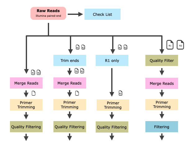
Once sequencing is complete, the raw FASTQ data must be processed before any meaningful analysis can be carried out. This step involves cleaning, organising and structuring the sequencing data so that it can be used to identify the species or taxa present in each sample.
Unlike wet-lab protocols, amplicon sequencing bioinformatics does not have a single universal approach. Each dataset has its own particularities including different sequencing platforms, primers, read lengths, error profiles and sample types. A fixed pipeline is rarely appropriate for all situations. Instead, the steps in the workflow must be carefully selected and sometimes adapted to match the nature and quality of the data.
Data processing in practice: servers and HPC clusters
In real projects, amplicon datasets are large enough that data processing is almost always run on a remote server or high-performance computing (HPC) cluster rather than a local laptop. On a cluster such as ETH Euler, each processing step is typically submitted as a separate job to a scheduler such as SLURM, rather than being chained into a single script. This modularity is deliberate: it lets you inspect intermediate output after each step, re-run only the stage that failed, and allocate appropriate compute resources to each task. Merging paired reads is fast and memory-light; chimera filtering on a large dereplicated dataset may require substantially more CPU time and memory. The hands-on exercises on this page are designed to run on the GDC server, which provides the same kind of controlled, shared environment.
Why not just use a fixed pipeline?
It is tempting to use an automated pipeline that performs all tasks with a single command. Tools such as QIIME2, mothur and USEARCH pipelines are powerful and widely used, and they can be the right choice in many situations. However, if you rely solely on a pipeline without understanding each step, you may miss important issues such as low-quality reads, poor primer trimming, or unusual chimera patterns. Understanding what each step does gives you the control and insight needed to troubleshoot problems and justify your choices when publishing results.
Hands-on Exercise: Data Processing
In this practical session, you will take your first steps working with real amplicon sequencing data. The aim is to explore and inspect raw reads from an environmental sample and begin processing them. You will work directly in the terminal using basic Linux commands and bioinformatics tools.
Step 1: Get Ready
We will be working on a remote server that hosts the necessary tools and environment.
## Log into the server
ssh guest??@gdc-vserver.ethz.ch
# Replace guest?? with the username assigned to you.

## Set up your working directory
mkdir -p ${HOME}/GDA/AmpSeq
cd ${HOME}/GDA/AmpSeq

## Download the example data
curl -O "https://www.gdc-docs.ethz.ch/GeneticDiversityAnalysis/GDA/data/SP05_R1.fastq.gz"
curl -O "https://www.gdc-docs.ethz.ch/GeneticDiversityAnalysis/GDA/data/SP05_R2.fastq.gz"
These are compressed FASTQ files containing paired-end sequencing reads from sample SP05.
You should see:
Step 2: Explore the Raw Data
Before diving into processing, it is helpful to understand what kind of data we are working with. Try answering the following questions using basic command-line tools.
Single-end or paired-end?
The _R1 and _R2 filenames indicate forward and reverse reads. This is paired-end data.
What is the read length?
zcat SP05_R1.fastq.gz | head -n 2 | tail -n 1
zcat SP05_R1.fastq.gz | sed -n '2~4p' | head -n 5 | awk '{ print length($0) }'
How many reads do we have?
Remember, FASTQ files have four lines per read.
What kind of sequences are these?
Extract a few reads and paste them into NCBI BLAST to identify them:
How many unique instrument IDs do we have?
Mixed IDs may indicate technical variation or pooling from different sequencing runs. If multiple IDs are present, consider accounting for them as potential batch effects.
curl -O "https://www.gdc-docs.ethz.ch/GeneticDiversityAnalysis/GDA/scripts/check_ids.sh"
bash check_ids.sh <(zcat SP05_R1.fastq.gz)
Challenge 1 — Explore the data further
Use command-line tools to answer: what platform was used, how long are the reads, how many reads are there, and what marker gene is this?
Solution
## QC report with FastQC
fastqc SP05_R*.fastq.gz

## Explore the sequence headers from the first and last records
zcat SP05_R1.fastq.gz | head -n 1
zcat SP05_R2.fastq.gz | head -n 1
# header first R1: @M01072:31:000000000-A7V7A:1:1101:16534:1596 1:N:0:1
# header first R2: @M01072:31:000000000-A7V7A:1:1101:16534:1596 2:N:0:1

zcat SP05_R1.fastq.gz | tail -n 4 | head -n 1
zcat SP05_R2.fastq.gz | tail -n 4 | head -n 1
# header last R1: @M01072:31:000000000-A7V7A:1:1103:27408:18721 1:N:0:1
# header last R2: @M01072:31:000000000-A7V7A:1:1103:27408:18721 2:N:0:1

## Read length
zcat SP05_R1.fastq.gz | head -n 2 | grep "@" -v | awk '{print length($1)}'
# read length: 288 nt => Illumina MiSeq PE-288 data

## Read count
zgrep -c "^+$" SP05_R[12].fastq.gz
# Both files: N = 10,000

## Identify sequences using BLAST
# Extract the top 3 sequences in FASTA format
zcat SP05_R1.fastq.gz | head -n 12 | grep "@M" -A 1 --no-group-separator | tr '@' '>'
# Based on BLAST results, this appears to be a 16S rRNA amplicon of bacteria.
Step 3: Merging Paired Reads
Now that we have explored the raw data, it is time to start processing it. The first step is to merge the paired-end reads, combining each forward (R1) and reverse (R2) read into a single longer sequence.
Why do we do this?
Amplicon sequencing often targets short regions of 250 to 500 bp, meaning the forward and reverse reads overlap in the middle. By aligning and merging the overlapping parts, we reconstruct the full-length amplicon. This improves data quality because mismatches in the overlap region highlight sequencing errors, and merging can help correct or remove them.
Tools for merging
Several tools are available for merging paired-end reads. In practice, merging is often handled within larger frameworks such as DADA2, VSEARCH, or QIIME2. In this exercise, we use FLASh (Fast Length Adjustment of SHort reads) as a standalone teaching example. FLASh is simple, fast, and produces useful diagnostic output that makes the merging step easy to inspect and understand. It works best when the overlapping region is at least 10 to 20 bp.
Key parameters to understand before running:
- Overlap (min and max): how much overlap between reads is required to merge them
- Mismatch tolerance: how many mismatches are allowed in the overlap region
- Read quality: low-quality bases in the overlap region can lead to poor merging
| FLASh (default) | Stats |
|---|---|
| Total reads | 10,000 |
| Combined reads | 4,583 |
| Uncombined reads | 5,417 |
| Percent combined | 45.8% |
The default merging run worked, but a success rate of around 46% is low. There was also a warning message:
[FLASH] WARNING: An unexpectedly high proportion of combined pairs (100.00%)
overlapped by more than 65 bp, the --max-overlap (-M) parameter.  Consider
increasing this parameter.
Warnings vs errors
A warning means the tool completed successfully but detected something unusual that may affect the results. It is asking you to think, not telling you that something broke. An error means the tool could not complete the task, usually due to a missing file, wrong parameter, or incompatible input.
This FLASh warning is a good example: the run finished and produced output, but the tool noticed that all merged pairs exceeded its default maximum overlap of 65 bp. This is useful diagnostic information. It tells you the parameter was poorly chosen for this dataset, and that you should adjust it before trusting the results. Ignoring warnings without reading them is one of the most common sources of silent errors in bioinformatics pipelines.
Let us try adjusting the parameters:
## Merge reads with relaxed parameters
flash SP05_R1.fastq.gz SP05_R2.fastq.gz --threads 1 \
      --min-overlap 8 \
      --max-overlap 288 \
      --max-mismatch-density 0.45
| FLASh (relaxed) | Stats |
|---|---|
| Total reads | 10,000 |
| Combined reads | 5,397 |
| Percent combined | 54.0% |
A bit better, but still not great. We could try relaxing the parameters further:
## Merge reads with very relaxed parameters
flash SP05_R1.fastq.gz SP05_R2.fastq.gz --threads 1 \
      --min-overlap 8 \
      --max-overlap 288 \
      --max-mismatch-density 0.95
| FLASh (very relaxed) | Stats |
|---|---|
| Total reads | 10,000 |
| Combined reads | 9,998 |
| Percent combined | 99.98% |
More reads merged, but is this actually better?
More is not always better
Lowering the stringency of merging parameters makes it easier for read pairs to merge, but increases the risk of joining reads that do not actually belong together or that contain more errors. A very high merge rate achieved by relaxing all constraints is not a sign of good data quality. Always inspect the QC report to evaluate the reliability of the merges.
Looking at the quality profile, read quality tends to decrease towards the end of the reads. This is a common issue with Illumina data.

Poor-quality bases at the ends of reads introduce mismatches in the overlap region, resulting in fewer or incorrect merges. To address this, we trim the low-quality ends of the reads before merging.
Conda environments
A Conda environment is an isolated software environment that bundles a tool together with all of its dependencies at specific versions. On shared servers, tools are often installed in named environments rather than system-wide to avoid version conflicts and ensure reproducibility.
Activating an environment with conda activate <environment-name> makes the software installed in that environment available in your current shell session. Your shell prompt will typically change to indicate the active environment. When you are finished, run conda deactivate to return to the base environment. Only one Conda environment can be active at a time.
We use fastp, a fast and flexible quality-filtering tool. It is installed inside a Conda environment on the server, which ensures all its dependencies are properly managed and isolated from other tools.
## Activate the fastp Conda environment
# See the note on Conda environments in the merging section above.
conda activate /usr/bin/condaenv/fastp
# Use `conda deactivate` to switch back when done.

fastp --version
fastp --help
## Trim forward reads to 240 bp
## The dominant amplicon is around 288 nt. Trimming R1 to 240 nt leaves a
## comfortable overlap of ~46 nt after merging, enough for reliable alignment
## while removing the lower-quality tail of each read.
fastp --max_len1 240 \
      --length_required 100 \
      --disable_adapter_trimming \
      --disable_quality_filtering \
      -i SP05_R1.fastq.gz -I SP05_R2.fastq.gz \
      -o SP05_R1_trim.fastq.gz -O SP05_R2_trim.fastq.gz
The selective options above focus fastp on length trimming only, leaving quality filtering and adapter trimming to dedicated steps later in the workflow. This makes each decision explicit and easier to audit.
| fastp (selective) | Stats |
|---|---|
| Reads before | 10,000 |
| Reads after | 9,996 |
| Reads filtered | 4 (too short after trimming) |
Now merge the trimmed reads:
## Merge trimmed reads
flash SP05_R1_trim.fastq.gz SP05_R2_trim.fastq.gz --threads 1 \
      --max-overlap 240
| FLASh (trimmed, selective) | Stats |
|---|---|
| Total reads | 9,996 |
| Combined reads | 9,667 |
| Percent combined | 96.7% |
Read loss accumulates across steps. Here we lost 4 reads in fastp and around 330 in merging, ending with 96.7% of the original data. This is normal and acceptable, as long as you understand why each loss occurred. Running QC before and after each step helps you make those judgements with confidence.
Challenge 2 — Redirect the fastp output to a log file
By default fastp writes its summary to the terminal. How would you save it to a file for later inspection?
Solution
## Option A: redirect to log file using tee
fastp --max_len1 240 \
  -i SP05_R1.fastq.gz -I SP05_R2.fastq.gz \
  -o SP05_R1_trim.fastq.gz -O SP05_R2_trim.fastq.gz 2>&1 | \
  tee log_fastp_230629.txt

## Option B: use fastp built-in HTML report
fastp --max_len1 240 \
  --html log_fastp_230629.html \
  --report_title "SP05 QC Report" \
  -i SP05_R1.fastq.gz -I SP05_R2.fastq.gz \
  -o SP05_R1_trim.fastq.gz -O SP05_R2_trim.fastq.gz
Now check the length distribution of the merged sequences:
infoseq -only -length out.extendedFrags.fastq | grep -v "Length" > amplicon_length.tmp
bash textHistogram.sh amplicon_length.tmp
The output shows amplicon lengths ranging from 211 to 468 nt. The vast majority are around 288 nt, as expected for this target region:
## Each # represents a bin of reads at that length.
## The dominant peak at 288 nt confirms the target amplicon size.
  286: #
  287: #####
  288: ##################################################
  289: #######
  290: #
Challenge 3 — Improve merging by also trimming R2
R1 and R2 reads have different error profiles. R2 generally deteriorates faster. Can you trim both reads separately and check whether merging improves?
Solution
fastp --max_len1 200 \
      --max_len2 180 \
      --length_required 100 \
      --disable_adapter_trimming \
      --disable_quality_filtering \
      -i SP05_R1.fastq.gz -I SP05_R2.fastq.gz \
      -o SP05_R1_trim.fastq.gz -O SP05_R2_trim.fastq.gz

flash SP05_R1_trim.fastq.gz SP05_R2_trim.fastq.gz
# N(merged): 9,836 (vs 9,667 with R1 trimming only)
With new read lengths of 200 and 180, the overlap is still 46 nt:
Primer Site Trimming
The primer sequences must be removed because they were added to the amplicon during PCR and are not part of the biological sequence being studied. Before trimming, the FLASh output file is renamed for clarity:
## Rename FLASh output
cp out.extendedFrags.fastq SP05_R12.fq
# We use R12 to indicate that R1 and R2 have been merged.

## Verify the number of sequences
grep "^+$" -c SP05_R12.fq
# N: 9,836
The primer sequences for this dataset are:
Forward Primer: 5'-CAGCNGCCGCGGTAANAC-3'    (18 nt)
Reverse Primer: 5'-GGACTACNNGGGTNTCTAATC-3' (21 nt)
Before trimming, we explore the primer sites to get a quick estimate of how many amplicons contain them. When searching for the reverse primer in merged reads, the reverse complement of the primer sequence must be used:
When using grep, note that real FASTQ files do not contain IUPAC ambiguity codes. Replace any ambiguous positions with bracket notation:
grep "CAGC[ACTG]GCCGCGGTAA[ACTG]AC" -c SP05_R12.fq
# N(forward primer found): 8,193 (83.3%)

grep "GATTAGA[ACTG]ACCC[ACTG][ACTG]GTAGTCC" -c SP05_R12.fq
# N(reverse primer found): 9,516 (96.7%)
Challenge 4 — Search for both primers in one grep command
The two primer searches above were run as separate commands. Can you combine them into a single grep call?
The grep approach provides only a quick estimate. We now use cutadapt for proper primer trimming, which handles IUPAC ambiguity codes and allows a configurable mismatch tolerance:
## Activate the cutadapt Conda environment
conda activate /usr/bin/condaenv/cutadapt
cutadapt --version
cutadapt --help

## Trim the forward primer
cutadapt -g CAGCNGCCGCGGTAANAC -e 0.1 -O 18 --trimmed-only \
         -o SP05_R12_trimPF.fq SP05_R12.fq
grep "^+$" -c SP05_R12_trimPF.fq
# N(after forward trim): 9,324 (94.8%)

## Trim the reverse primer
cutadapt -a GATTAGANACCCNNGTAGTCC -e 0.1 -O 21 --trimmed-only \
         -o SP05_R12_trimPF_trimPR.fq SP05_R12_trimPF.fq
grep "^+$" -c SP05_R12_trimPF_trimPR.fq
# N(after reverse trim): 9,304 (99.8%)
Overall, primer trimming results in a loss of about 5.4% of amplicons. This two-step approach is useful for understanding what happens at each stage, but in practical pipelines both primers can be trimmed in one step.
Challenge 5 — Trim both primers in a single cutadapt command
The two-step trimming above runs cutadapt twice. Can you achieve the same result in one command, discarding any reads where neither primer was found?
Solution
cutadapt -g CAGCNGCCGCGGTAANAC \
         -a GATTAGANACCCNNGTAGTCC \
         -e 0.1 -O 15 \
         --discard-untrimmed \
         -o SP05_R12_trimmed.fq SP05_R12.fq
-g and -a in one call trims the forward and reverse primers in a single pass. --discard-untrimmed drops any read where neither adapter was detected.
Clustering
We use USEARCH for clustering and denoising. The key decision at this stage is whether to produce OTUs (97% similarity clusters) or zOTUs/ASVs (exact sequences after error correction).
Chimera removal
Before clustering, it is important to understand what chimeras are and why they must be removed. Chimeras are artificial sequences generated during PCR when an incomplete extension product from one cycle acts as a primer in a subsequent cycle and is extended using a different template. The result is a hybrid sequence that does not correspond to any real organism. If left in the dataset, chimeras inflate diversity estimates and can appear as novel or unclassified taxa. Both USEARCH and VSEARCH implement reference-based and de novo chimera detection, and chimera filtering is a standard step in all modern amplicon workflows.
FASTQ to FASTA conversion
Before clustering, USEARCH requires FASTA input. We convert the trimmed FASTQ file using usearch -fastq_filter, which also applies a final quality pass:
## Convert FASTQ to FASTA
usearch -fastq_filter SP05_R12_trimPF_trimPR.fq \
        -fastaout SP05_R12_trimPF_trimPR.fa
grep "^>" -c SP05_R12_trimPF_trimPR.fa
# N: 9,304
Dereplication and clustering
## Dereplicate amplicons (collapse identical sequences)
usearch -fastx_uniques SP05_R12_trimPF_trimPR.fa \
        -fastaout SP05_Uniques.fa \
        -sizeout

# Stats:
# 9,304 seqs, 4,644 uniques, 3,330 singletons (71.7%)
# Min size 1, median 1, max 221, avg 2.00

## Option A: Create 97% similarity clusters (OTUs)
usearch -cluster_otus SP05_Uniques.fa \
        -otus SP05_OTU.fa \
        -minsize 2

## Option B: Create error-corrected zero-radius OTUs (zOTUs, equivalent to ASVs)
usearch -unoise3 SP05_Uniques.fa \
        -zotus SP05_zOTU.fa \
        -minsize 3

grep "^>" -c SP05_zOTU.fa
# 636 zOTUs
To obtain count tables, we map the trimmed amplicons back to the clusters:
usearch -otutab SP05_R12_trimPF_trimPR.fa \
        -otus SP05_zOTU.fa \
        -otutabout SP05_zOTU.tab
# 7,019 / 9,304 mapped to zOTUs (75.4%)
Taxonomic Assignments
We now have a count table with zOTUs as rows and samples as columns. The next step is to assign taxonomic identities to each zOTU using a reference database.
Classification methods
Several approaches are in common use and it is worth knowing their differences:
SINTAX (used here) is a k-mer bootstrap classifier that assigns taxonomy by comparing query sequences against an annotated reference database and reporting confidence values at each rank. It is fast and works well with the USEARCH/VSEARCH ecosystem.
Naive Bayes classifiers, as implemented in QIIME2 (via the q2-feature-classifier plugin), train a probabilistic model on a reference database and assign taxonomy based on the posterior probability of each classification. These are widely used and perform well at the genus level for common marker genes.
BLAST with a lowest common ancestor (LCA) approach searches for close matches in a reference database and assigns the most specific rank at which all top hits agree. This is more conservative than direct top-hit assignment and reduces spurious species-level classifications.
The choice of classifier and reference database together determine what taxonomy your zOTUs receive. Different combinations can yield different results, sometimes at relatively high ranks.
Reference database
The RDP 16S reference database used in this exercise is pre-installed on the GDC server. You do not need to download it.
## Reference database path on the GDC server
REF="/usr/data/rdp_16s_v18.fa"

## Check the reference
head -n 4 ${REF}
grep ">" -c ${REF}
# N = 10,049

## Run taxonomic prediction with SINTAX
usearch -sintax SP05_zOTU.fa \
        -db ${REF} \
        -strand both \
        -sintax_cutoff 0.85 \
        -tabbedout SP05_zOTU_RDP.tax

## Example: inspect the most abundant zOTU
grep "Zotu1" -w SP05_zOTU_RDP.tax
# => d:Bacteria,p:Acidobacteria,c:Acidobacteria_Gp4,g:Gp4
We can check this assignment using NCBI BLAST. For 16S sequences, the RefSeq RNA database is more informative than the full nt collection:
>Zotu1
GGGGGGAGCAAGCGTTGTTCGGATTTACTGGGCGTAAAGGGCGCGTAGGCGGTCAGCACAAGTCAGTTGTGAAATCTCCG
GGCTTAACTCGGAAAGGTCAACTGATACTGTGCGACTAGAGTGCAGAAGGGGCAACTGGAATTCTCGGTGTAGCGGTGAA
ATGCGTAGATATCGAGAGGAACACCTGCGGCGAAGGCGGGTTGCTGGGCTGACACTGACGCTGAGGCGCGAAAGCCAGGG
GAGCGAACGG
Top 5 BLAST hits:
| Accession | Species | Coverage | Identity | Taxonomy |
|---|---|---|---|---|
| NR_151987.1 | Brevitalea aridisoli | 100% | 93.6% | Bacteria;Acidobacteria;Blastocatellia;Blastocatellales;Pyrinomonadaceae;Brevitalea |
| NR_151988.1 | Brevitalea deliciosa | 100% | 93.6% | Bacteria;Acidobacteria;Blastocatellia;Blastocatellales;Pyrinomonadaceae;Brevitalea |
| NR_151986.1 | Arenimicrobium luteum | 100% | 93.6% | Bacteria;Acidobacteria;Blastocatellia;Blastocatellales;Pyrinomonadaceae;Arenimicrobium |
| NR_146026.1 | Tellurimicrobium multivorans | 98% | 91.5% | Bacteria;Acidobacteria;Blastocatellia;Blastocatellales;Blastocatellaceae;Tellurimicrobium |
| NR_146021.1 | Stenotrophobacter namibiensis | 98% | 91.5% | Bacteria;Acidobacteria;Blastocatellia;Blastocatellales;Blastocatellaceae;Stenotrophobacter |
The top 5 hits agree on:
As an alternative, SILVA's SINA aligner can be used for classification:
# SINA result for zOTU1:
# d:Bacteria;p:Acidobacteriota;c:Blastocatellia;o:Pyrinomonadales;f:Pyrinomonadaceae;RB41
The results largely agree, except for the order-level label. This is not a simple error in either database. NCBI RefSeq follows a classification in which Pyrinomonadaceae is a family within the order Blastocatellales, while SILVA follows a scheme in which the same clade is elevated to an independent order, Pyrinomonadales. Both are valid positions reflecting an unresolved question in bacterial systematics. The discrepancy illustrates how nomenclatural and classificatory decisions by database curators can affect annotation results independently of any sequencing or algorithmic issue.
Taxonomic assignments are always uncertain
The taxonomic classification of OTUs and zOTUs carries uncertainty from at least three independent sources. First, no reference database is complete or error-free, so a query sequence may match an incorrectly annotated reference or find no close match at all. Second, the amplicon may be too short or too conserved to resolve assignments below a certain rank. Third, reference databases differ in the nomenclature and circumscription they adopt, meaning the same sequence can receive different valid labels depending on which database is used, as the Blastocatellales/Pyrinomonadales discrepancy above illustrates. Assignments should never be treated as ground truth, and the choice of reference database can materially affect the results.
Data Analysis
For the exercises, download and unzip the R script, the data, and the helper functions:
## Set up working directory
getwd()
setwd("~/GDA/")
# dir.create("~/GDA/", recursive = TRUE)

## Download and unzip the exercise files
data.url <- "https://www.gdc-docs.ethz.ch/GeneticDiversityAnalysis/GDA/data/AmpSeqExample.zip"
download.file(data.url, destfile = "AmpSeqExample.zip")
unzip("AmpSeqExample.zip")

## Check the files
list.files("AmpSeq")
# AmpSeq/AmpliconSeq_DataAnalysis.Rmd  : RMarkdown script for the exercises
# AmpSeq/Chaillou2015.Rdata : input dataset
# AmpSeq/graphical_methods.R: helper functions

## Clean up the zip file
file.remove("AmpSeqExample.zip")

## Open the R script
setwd("~/GDA/AmpSeq/")
file.edit("AmpliconSeq_DataAnalysis.Rmd")
Additional Resources
AmpSeq data preparation workflows
- UPARSE and UNOISE (USEARCH)
- VSEARCH
- QIIME2
- mothur
- DADA2 pipeline
- OBITools
- nf-core/ampliseq (Nextflow)
Data analysis
- Phyloseq: analysis of microbiological communities
- microbiome R package
- ampvis2
- vegan: community ecology in R
- mixOmics
Reference databases