Massively Parallel Sequencing

Learning Objectives
Main
- Understand the basic principles and differences between massively parallel sequencing (MPS) platforms.
- Understand sample indexing and sequence read types.
Minor
- Know the common raw data file formats produced by different sequencing platforms.
- Understand the importance of read data archives and know where to submit or retrieve sequencing data.
- Understand the advantages, limitations and applications of MPS in genomics, transcriptomics and metabarcoding.
- Recognise common sequencing artefacts such as adapter contamination and understand how to detect and remove them.
Massively Parallel Sequencing
Massively parallel sequencing (MPS) refers to any of several high-throughput approaches to DNA sequencing that use the concept of massively parallel processing — sequencing millions to billions of DNA fragments simultaneously rather than one at a time.
MPS and NGS
We use the term massively parallel sequencing (MPS) because it is a more general term that also includes newer sequencing technologies. Next-generation sequencing (NGS) technically refers to PCR-based sequencing technologies such as Roche 454 and Illumina, while single-molecule sequencing platforms such as PacBio and Oxford Nanopore are often described as third-generation or single-molecule sequencing. We keep it simple and use MPS throughout.
Biological and medical science has been, and continues to be, revolutionised by rapid advances in modern DNA sequencing technologies. The ease of data generation has shifted the main research focus from individual loci to whole genomes, increased sample numbers dramatically, created new demands for data management, and fundamentally changed data analysis. As a result, nucleotide sequence archives such as ENA and NCBI SRA are growing daily.
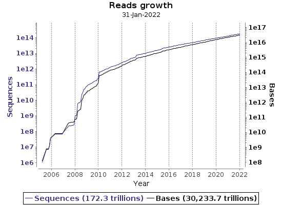
ENA regularly publishes statistics on data growth.
Sequencing Technologies
First Generation Sequencing
Second Generation Sequencing
- 454 Sequencing
- Ion Torrent
- Illumina Sequencing Technology
- Element Biosciences AVITI / Avidity Base Chemistry Infographic
- Singular Genomics
Third Generation Sequencing (Single Molecule)
Genome Mapping
Yes we can, but should we?
High-throughput sequencing is a powerful tool, but generating large amounts of data without a clear purpose or understanding leads to many challenges. Sequencing efforts guided by clear hypotheses and research objectives will ensure that the data generated is relevant and makes a meaningful scientific contribution. Different sequencing technologies have different strengths and weaknesses. Choosing the right technology based on the specific needs of your study, including read length, accuracy, bias and coverage, is essential for accurate data interpretation.
Platform Comparison
There are many reports comparing MPS technologies, but they are often out of date by the time they are published. Sequencing technology develops rapidly and it is difficult to keep up. The following is a rough and personal guide based on the platforms most commonly used at the GDC.
| Platform | Strengths | Limitations |
|---|---|---|
| Illumina | Very high accuracy and throughput, large user community, mature ecosystem | Short read lengths limit resolution of repetitive regions |
| BGI | Competitive cost and high throughput | Different performance characteristics to other platforms; smaller user community |
| Element Biosciences (AVITI) | Outstanding accuracy, now exceeding Illumina in several benchmarks, competitive cost | Still building market presence and support ecosystem |
| Singular Genomics | Competitive short-read platform with strong accuracy | Taken private in early 2025 and currently focused on spatial multiomics rather than standard sequencing; availability as a sequencing service may be limited |
| PacBio (HiFi) | Long reads with very high consensus accuracy | Higher cost per base; requires higher DNA input quantity |
| Oxford Nanopore (ONT) | Ultra-long reads, real-time sequencing, portable | Higher per-base error rate than short-read platforms; requires intact high molecular weight DNA |
Choosing the right technology
The question and all available resources should determine the sequencing technology, not just cost. There is no benefit to aiming for long reads if the starting DNA is highly fragmented or available only in small quantities. Element Biosciences has recently emerged as a strong competitor to Illumina for short-read applications, with independent benchmarks showing improved accuracy particularly in homopolymers and repetitive regions. Singular Genomics was taken private in early 2025 and is currently focused on spatial multiomics; the situation may have changed by the time you read this, so check current sources before drawing conclusions.
Raw Data File Formats
Illumina sequence reads are provided as demultiplexed FASTQ.gz files. FASTQ combines sequence and per-base quality scores in a simple text format; see Biocomputing: Basics for details on the format.
PacBio sequence reads are provided as FASTQ, HiFi (circular consensus sequence, CCS) FASTQ, or BAM files. HiFi reads are highly accurate: shorter fragments are read multiple times by circling them through the polymerase during a run, and accuracy increases with each pass, typically reaching over 99.9% at sufficient coverage.
Oxford Nanopore (ONT) raw data are provided as FAST5 (older) or POD5 (newer) files and must be base-called using tools such as Dorado to obtain FASTQ files.
FASTQ is the common format for sharing sequencing read data. For Illumina paired-end (PE) runs, you will have two FASTQ files per sample (R1 and R2). For single-end (SE) runs, Illumina, PacBio and Nanopore data, you will have one FASTQ file per sample.
Data Archives
Sharing your raw sequencing data with the scientific community is both good practice and, for publicly funded research, often a requirement. Submit your raw data to one of the three internationally recognised repositories. The European Nucleotide Archive (ENA), the NCBI Sequence Read Archive (SRA), and the DNA DataBank of Japan (DDBJ) are all part of the International Nucleotide Sequence Database Collaboration and exchange data regularly.
- International Nucleotide Sequence Database Collaboration
- European Nucleotide Archive (ENA)
- ENA: Guidelines and Tutorials
- NCBI: Sequence Read Archive (SRA)
For other data types such as processed files, metadata, and analysis code, general research repositories are a good option:
Choosing the right repository
The best repository depends on the type of data, the subject area, and the specific requirements for storage and sharing. Review the features and policies of each repository before deciding which one best suits your needs.
Challenges
For the following challenges, we assume you are familiar with NCBI BLAST searches. If not, NCBI BLAST tutorials and NCBI webinars are a good place to start.
First, we generate two 29nt random DNA sequences with a GC content of 50% and 20%. You can use the Random Sequence Generator from molbiotools, write your own, or use the example below.
Approaches to Generating a Random Sequence
There is more than one way to generate a random nucleotide sequence. The three approaches below produce equivalent output but differ in flexibility and context. Use whichever you are most comfortable with, and take a moment to read through the others.
Bash: quick and direct
A compact command-line solution. Note that tr -dc 'AACTTG' does not produce equal nucleotide frequencies because A and T appear twice in the character class.
rm -f RandomSequence.fa
echo ">RandomSequence (29nt)" > RandomSequence.fa
cat /dev/urandom | tr -dc 'AACTTG' | fold -w 29 | head -n 1 >> RandomSequence.fa
cat RandomSequence.fa
R: a single reusable function
Using sample() with a prob argument gives explicit control over nucleotide frequencies. The function prints directly to the console in FASTA format.
generate_fasta <- function(header = "RandomSequence", length = 29,
                           frequencies = c(0.25, 0.25, 0.25, 0.25)) {
  nucleotides <- c("A", "C", "G", "T")
  sequence    <- paste(sample(nucleotides, length, replace = TRUE, prob = frequencies),
                       collapse = "")
  cat(paste0(">", header, "\n", sequence, "\n"))
}

# AT-rich example: 40% A, 10% C, 10% G, 40% T
generate_fasta(header = "RandomSequence", length = 29,
               frequencies = c(0.4, 0.1, 0.1, 0.4))
R with seqinr: writing directly to a FASTA file
Useful when downstream tools expect a FASTA file on disk. The seqinr package handles formatting and line wrapping. This version also embeds sequence metadata in the header.
SeqN <- 3             # Number of sequences
SeqL <- 29            # Sequence length
NucF <- rep(0.25, 4)  # Nucleotide frequencies: A T C G

set.seed(060623)
DNA         <- c("A", "T", "C", "G")
GCcontent   <- sum(NucF[3:4]) * 100
FastaOutput <- "RandomSequence.fasta"
if (file.exists(FastaOutput)) unlink(FastaOutput)

for (i in seq_len(SeqN)) {
  header <- paste0("RandomSequence_", i, " L:", SeqL, "nt GC:", GCcontent, "%")
  seq    <- paste(sample(DNA, SeqL, replace = TRUE, prob = NucF), collapse = "")
  seqinr::write.fasta(seq, header, FastaOutput, open = "a", nbchar = 60, as.string = TRUE)
}
Things to notice
- The bash version silently skews nucleotide frequencies because of the repeated characters in the
trcharacter class. Can you fix it? - All three use random sampling under the hood; they differ in where the output goes and how much control you have over the parameters.
- Only the
seqinrversion writes a file directly and embeds metadata in the header. The others print to the console or require a shell redirect.
Possible sequence example:
>RandomSequence_01_L29_GC50
CGTAAGGCCATTGCGAATACCAGGTATCG
>RandomSequence_02_L29_GC20
AAACTGTTAAAAAATCGTGTCTTTACAAT
Challenge 1: Identify the sequence file format
What is the text-based format representing these two nucleotide sequences called, and what would be an appropriate file extension?
Solution
The format is called FASTA (see Biocomputing: Basics for more detail). The file extension should be .fa or .fasta. If the sequences are aligned, the extension .afa is commonly used.
Possible file name: RandomSequences.fa
Challenge 2: Sequence space and probability
How many ways are there to build a 29nt long sequence? What is the probability of generating exactly the same sequence twice? How does GC content affect this probability?
Solution
There are 4 possibilities (nucleotides) for each of the 29 positions, resulting in 4^29 = 2.88 x 10^17 possible sequences. The likelihood of generating the same sequence twice is therefore extremely small.
A lower GC content reduces sequence complexity, slightly increasing the chance of chance matches, as we will see in the next challenge. Sequences skewed strongly towards AT or GC occupy a smaller fraction of total sequence space and are more likely to share short identical stretches with other sequences.
Now add the following unknown sequence to the two randomly generated sequences:
Challenge 3: Calculate GC content
What is the GC content of the mystery sequence? You can calculate it in bash, R, or both.
Solution
The GC content is approximately 52% (15 G/C out of 29 nucleotides), similar to random sequence #1.
Simple bash:
# Total length
echo -n "AATGATACGGCGACCACCGAGATCTACAC" | wc -c

# Alternative using string length
string="AATGATACGGCGACCACCGAGATCTACAC"
echo "Length: ${#string}"

# Count Cs and Gs (remove A and T, count remaining)
echo -n "AATGATACGGCGACCACCGAGATCTACAC" | sed -E 's/A|T//g' | wc -c

# GC percentage
echo "scale=2; 15/29*100" | bc
More robust bash:
string="AATGATACGGCGACCACCGAGATCTACAC"
string=$(echo "$string" | tr '[:lower:]' '[:upper:]')
string_length=${#string}
count_GC=$(echo "$string" | grep -o '[CG]' | wc -l)
percentage_GC=$((count_GC * 100 / string_length))
echo "GC content: $percentage_GC%"
R function:
GCcontent <- function(sequence){
  sequence_caps   <- toupper(sequence)
  split_sequence  <- strsplit(sequence_caps, "")[[1]]
  sequence_length <- length(split_sequence)
  gc_content      <- sum(split_sequence == "C" | split_sequence == "G")
  return(paste("GC content is", round((gc_content/sequence_length)*100, 1), "%"))
}
GCcontent("AATGATACGGCGACCACCGAGATCTACAC")
The next challenges require you to use external tools and interpret results independently. There is no single correct answer, and part of the exercise is forming and testing your own expectations before looking at the output.
Next, we search the largest available collection of nucleotide sequences to look for similar known sequences. Compare all three sequences against the NCBI nt BLAST database.
Challenge 4a: Form your expectations before BLASTing
Before running BLAST, write down what results you expect for each of the three sequences. Consider GC content, sequence complexity, and whether any sequence might have a non-random origin.
Solution
Seq1 (GC 50%): A well-balanced random sequence should not produce a perfect hit. The sequence is short and the database is large, so occasional weak partial hits cannot be excluded, but 100% coverage and 100% identity would be surprising.
Seq2 (GC 20%): A lower-complexity sequence may produce some hits due to reduced sequence diversity, which can inflate apparent similarity. We might see more partial hits than with Seq1.
Seq3 (mystery): It is unclear. If truly random, results should resemble Seq1. If there are many perfect hits across unrelated organisms, the sequence may not be random at all.
Now compare all three sequences against the NCBI nt BLAST database.
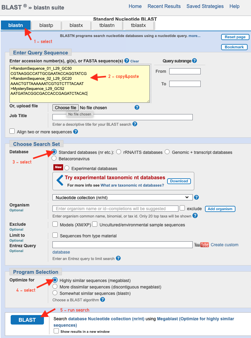
- Choose "Nucleotide BLAST"
- Paste all three sequences into the "Enter Query Sequence" field
- Choose database "Standard databases (nr etc.)"
- Select "megablast"
- Run BLAST
Challenge 4b: Interpret your BLAST results
Interpret your BLAST results carefully and compare with your expectations. Do you have any idea what the mystery sequence could be?
Solution
Seq1: As expected, no perfect hit with 100% coverage and 100% identity. Some partial hits with mismatches are possible but not biologically meaningful.
Seq2: Similar results to Seq1. Low-complexity sequences do not necessarily produce better hits than balanced ones.
Seq3: Unlike Seq1, BLAST returns numerous perfect hits (100% similarity, 100% coverage) across a wide range of unrelated organisms: carp, sea anemone, pineapple, fungi, bacteria, and SARS-CoV-2. This is not a coincidence. A sequence found identically in organisms this evolutionarily distant is almost certainly not a biological coding or regulatory sequence.
The mystery sequence is an Illumina Nextera adapter — an oligonucleotide added to DNA fragments during library preparation to enable sequencing. It appears in NCBI because many submitted sequences were not fully cleaned before deposition. Adapter contamination should always be removed before assembly or downstream analysis using tools such as fastp, Cutadapt, or Trimmomatic.
See the Illumina adapter sequences linked in Resources and BLAST a few more to confirm.
Challenge 5: A 46nt mystery sequence
Here is a 46nt sequence. BLAST it against the NCBI nt database. What do you find, and what do you conclude?
Challenge 5a: Hits and biological sense
BLAST returns perfect or near-perfect hits across unrelated organisms including plants such as Triticum monococcum. At first glance this looks like a biologically conserved sequence. However, these organisms share no obvious biological reason to conserve such a sequence, and the hits are scattered across genome assemblies rather than in functional gene regions. This pattern is the first sign that the hits are not biological.
Challenge 5b: Most likely explanation
The sequence is the PacBio SMRTbell adapter (ATCTCTCTCTTTTCCTCCTCCTCCGTTGTTGTTGTTGAGAGAGAT). A Google search returns the official PacBio barcoded adapter file directly: PacBio-Barcoded-Adapters.xlsx.
The hits in genome assemblies are almost certainly adapter contamination in publicly deposited sequences: submitters used PacBio sequencing and did not fully remove adapter sequences before assembly and deposition. This is a known problem in public databases and a reminder that even curated repositories such as NCBI are not free of artefacts.
Challenge 6: A third mystery sequence
Here is another 29bp sequence. Any idea what it might be?
Solution
Starting with Google returns no obvious clues. BLAST produces hits across rodents, primates, nematodes, moths, diatoms, bacteria and viruses, but local alignments consistently cover positions 4 to 29, not the full length.
Searching a shorter internal fragment (TGTACTTCGTTCAGTTACGTATTGCT) in Google returns a result from FreePatentsOnline. This is an Oxford Nanopore adapter sequence.
More information on ONT adapter sequences is available from the Nanopore Community.
Know what you don't know.
These three adapter challenges teach a lesson that goes beyond simply cleaning your reads. Adapter sequences left in your data are not neutral: because the same adapter appears on many reads, assemblers treat them as genuine overlapping sequence and may join unrelated contigs through them. The result can be a chimeric assembly with a misleadingly low contig count and inflated N50. An assembly that looks impressive by standard metrics may be structurally wrong. Fewer contigs is not always better.
Challenge 5 illustrates a second consequence: contaminated sequences submitted to public databases become everyone's problem. A BLAST search against NCBI is only as reliable as the sequences it contains, and as you have seen, adapter sequences from PacBio library preparation have made it into wheat genome assemblies. Hits to unrelated organisms are not always biology.
The broader lesson is this: understanding your data means understanding how it was generated, from DNA extraction and library preparation through sequencing chemistry and adapter design. Skipping that understanding does not make the artefacts disappear. It just makes them harder to find.
Resources
Help
Reading