Data Preparation
Experimental / Sampling Design
The sampling design is simple. There are 48 samples in total. The study compares apples from two different management groups (treatment). For each treatment, they took 6 tissue samples from four apples.
N(samples): 2 treatments x 4 replicates x 6 tissues = 48
The experimental design is well desribed in the paper.
Four apples, weighing 190 ± 5 g, were selected from each of the two management groups and each apple was divided into six tissues with the following weights: stem: 0.2 g, stem end: 2 g, peel: 9 g, fruit pulp: 12 g, seeds: 0.2 g, and calyx end: 3 g. Thus, each tissue was represented by four replicates, where each replicate consists of the respective tissue of one apple. source: Wassermann et al. 2019
The way I understand it, there are 4 data points for each treatments and tissue. This is important because my understanding does not correspond with the results of the diversity analysis as shown in figure 2 (see alpha diversity). The design also indicates that the different tissue samples are not independent samples since they derived from the same apple. This is important for the comparison between treatment where all samples are grouped together.
Heterogeneous Sample Preparation
There are three major concerns I have about pooling samples from different tissues to study treatments effects. (i) The tissue sample weight differs by a factor of 60. This could be problematic for comparisons since sample collection (e.g., genomic DNA concentration) can influence the variability in microbial communities (Multinu et al. 2018). (ii) Data obtained from samples using different DNA extraction protocols is problematic. DNA extraction method can influence the observed bacterial diversity (e.g., Teng et al. 2018) and bias comparisons. (iii) Another good reason for not combining (exterior and interior) tissue samples is the post-harvest treatment of non-organic apples (see below).
Management Groups
The studies focused on Arlet (Swiss Gourmet) apples from two different management groups: organic and conventional. The comparison between treatment is a central part of the study. The fact that the conventional grown apples underwent further treatment after the harvest while the organic apple did not is clearly described in materials and methods but ignored in the interpretation.
In contrast to the organically produced apples, they underwent the following post-harvest treatments: directly after harvest, apples were short-term stored under controlled atmosphere (1–2◦C, 1.5–2% CO2), washed and wrapped in polythene sheets for sale. Both apple management groups (“organic” and “conventional”) were transported to laboratory immediately and processed under sterile conditions. source: Wassermann et al. 2019
Treatment Bias
Based on a paper by Buchholz et al. (2018) it might be fair to assume that the post-harvest handling of the non-organic apples could have influenced their microbiota composition at least regarding communities associated with exterior tissue samples like peel, calyx, or stem. The authors, however, completely ignore this possibility and conclude that the difference they found between treatments is caused by the management practise. I think it is not legitimate to simplify the comparison to organic versus non-organic apples!
Raw Data
The authors stated that the raw sequence files to support their study are available from the ENA.
The raw sequence files supporting the findings of this manuscript are available from the European Nucleotide Archive (ENA) at the study Accession Number: PRJEB32455. source: Wassermann et al. 2019
Because Illumina MiSeq paired-end 250nt was used for sequencing, I expected to get two files (R1 and R2) per sample. To my surprise, there was only one sequence file per sample available. I asked the authors for help and got the following answer:
We receive our reads from the sequencing company in form of one forward file and one reverse file containing all reads of the whole pool, which, in this case, contained other samples as well. Data are demultiplexed after joining reads and removing barcodes. Those sequences are than provided in ENA. Thus, I cannot sent you the raw files from this pool. I´m sorry for that. source: personal communication with Brigit Wassermann
Ihe raw MiSeq reads are not available. The authors provide merged reads but provide little detail about the demultiplexing or merging process.
Raw sequence data preparation and data analysis was performed using QIIME 1.9.1 (Caporaso et al., 2010). After paired reads were joined and quality filtered (phred q20), chimeric sequences were identified using usearch7 (Edgar, 2010) and removed. source: Wassermann et al. 2019
While we can discuss the meaning of “raw data” but I am missing clarity here.
What are raw data
Raw data from an Illumina MiSeq paired-end data run would comprise a forward (R1) and a reverse (R2) read if standard Illumina adaptors were used and the samples are de-muliplex by the system. Customisation with barcoded primers might not alow an automated demuliplexing. Uploading demultiplexed reads are therfore justified but this needs to be clearly indicated and the process clearly descripted.
What does this matter? Merging forward (R1) and reverse (R2) read can have an influence on the data removed. It is not uncommon that removing the qualitatively bad ends of reads increases the merging efficiency. Here an exmaple from a 16S amplicon sequenceing data set produced at the GDC:
# R1:  0nt; R2:  0nt => 50.68% (merging efficiency)
# R1:  5nt; R2: 10nt => 95.62%
# R1: 10nt; R2: 20nt => 98.55%
# R1: 15nt; R2: 30nt => 90.75%
The read-merging step is unclear and therfore the adjusted quality scores of the merged data not reproducible.
Data Prepartion
I believe that we should keep as much data during the data process as possible. If we remove data during the data processing steps (e.g., filtering, merging) we should document it. I have no troubles to remove data as long as I have good reasons for doing so.
Negative and Positive Controls
The study does not include any negative controls. Therefore, we cannot estimate contamination. This is especially important because the samples are most likely processed by different experimentator (i.e. students) with different lab experiences. There are also no positive controls included in the study.
Data Preparation
I downloaded 48 fastq.gz files from the European Nucleotide Archive (ENA) using study number PRJEB32455. In total, there are 8,248,796 amplicon sequences (merged reads). I compared the amplicon length distribution with expected distribution obtain from in-silico PCR results based on SILVA 16S database (version 128) and NCBI bacteria genomes (version July2019).
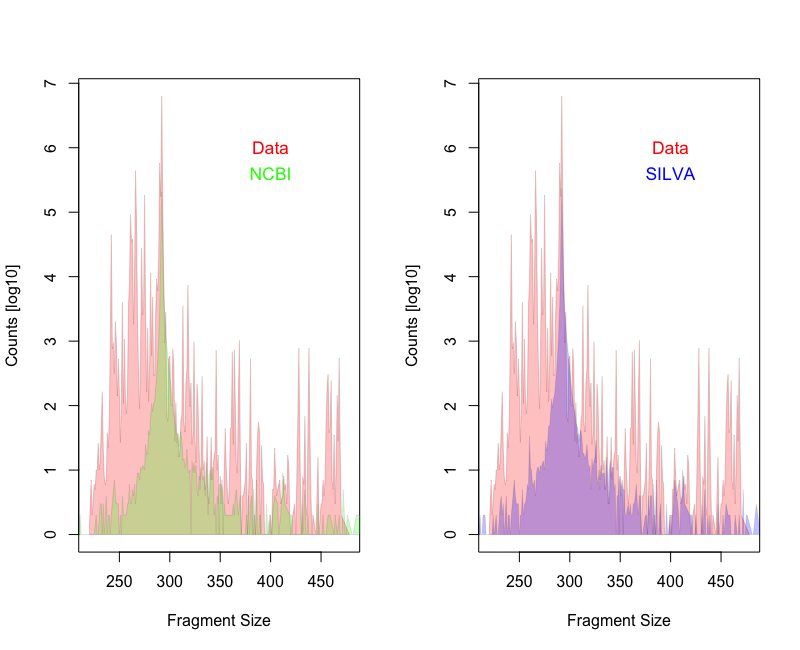

While the mean amplicon length is similar for the expected (292nt) and the observed (289nt) the distribution is not. There are many more shorter fragments present in the apple data.
Primer Trimming
The downloaded sequences still contained the primer region. I did not find any information about primer removal in the paper. I therefore assume, the primer region was not trimmed prior to clustering.
For culture-independent Illumina MiSeq v2 (250 bp paired end) amplicon sequencing, the primers 515f – 806r (Caporaso et al., 2010) were used to amplify the 16S rRNA gene using three technical replicates per sample. source: Wassermann et al. 2019
I assume the original primer 515F and 806R have been used for the amplification of the V4 region of the 16S SSU rRNA (Caporaso et al. (2011))
>515f
GTGCCAGCMGCCGCGGTAA
>806r
GGACTACHVGGGTWTCTAAT
I used usearch to remove the primer region allowing maximum 1 mismatch but not at primer end.
usearch v11.0.667_i86linux64
Amplicon range: 100-2000
Number of mis-matches: 1 / not at the end
Coverage: full-length
Wildcards enabled: IUPAC codes
I allowed one mismatch to reduce the data loss at this step.
# Mismatches: 0 =>  7,713,726
# Mismatches: 1 =>    335,973
# Mismatches: 2 =>     16,135
# Mismatches: 3 =>      7,082
Quality Filtering
In a next step, I quality filtered the data using Prinseq.
PRINSEQ-lite 0.20.4
Size Range: 100-600
GC Range: 30-70
Min Q Mean: 20
Number of Ns: 0
Low Complexity: dust / 30
OTU Clustering / Amplicon Sequence Variants
I used two different approaches to get operational taxonomic units (OTUs): UPARSE (Edgar 2016a) and UNOISE (Edgar 2016b). I also did some additional cluster for the zero OTUs (ZOTUs) to account for possible early PCR errors.
After removing chimeric, mitochondrial and chloroplast sequences, the overall bacterial community of all apple samples, assessed by 16S rRNA gene amplicon sequencing, contained 6,711,159 sequences that were assigned to 92,365 operational taxonomic units (OTUs). source: Wassermann et al. 2019
Number of OTUs     : 3,124 (308 Mitochondria / 52 Chloroplast)
Number of ZOTUs    : 3,182 (210 Mitochondria / 70 Chloroplast)
Although the amplicon sequence variant approach (ZOTU) has a tendency to overestimate the number of OTUs, I still found 30 times fewer OTUs than the authors. I cannot explain the difference because we both used USEARCH.
Representative sequences were aligned, open reference database SILVA (ver128_97_01.12.17) was used to pick operational taxonomic units (OTUs) and de novo clustering of OTUs was performed using usearch. source: Wassermann et al. 2019
The data processing of the provided merged reads removed on average 2.5% of the data. The data loss and the average amplicon size were steady between samples. The data processing of the provided merged reads removed on average 2.5% of the data. The data loss and the average amplicon size were steady among the samples. Sequence depth ranged from 18k to 428k with fruit pulp samples being at the lower range of the spectrum and calyx samples at the top.
Data-Prep Statistic
| Sample | Merged | Primer | Clean | MeanLength | D% |
|---|---|---|---|---|---|
| H-Stem-a | 205945 | 201311 | 201311 | 251.7 | 97.7 |
| H-Stem-b | 231409 | 223661 | 223661 | 251.7 | 96.7 |
| H-Stem-c | 217307 | 211969 | 211969 | 250.1 | 97.5 |
| H-Stem-d | 218388 | 214743 | 214743 | 251.5 | 98.3 |
| C-Stem-a | 181279 | 174667 | 174667 | 252.1 | 96.4 |
| C-Stem-b | 144427 | 141113 | 141113 | 252.4 | 97.7 |
| C-Stem-c | 372408 | 363099 | 363099 | 249.9 | 97.5 |
| C-Stem-d | 385316 | 375813 | 375813 | 252.5 | 97.5 |
| H-StemEnd-a | 221403 | 206834 | 206834 | 253.0 | 93.4 |
| H-StemEnd-b | 320614 | 310926 | 310926 | 251.9 | 97.0 |
| H-StemEnd-c | 86899 | 84075 | 84075 | 252.3 | 96.8 |
| H-StemEnd-d | 197981 | 194176 | 194176 | 251.9 | 98.1 |
| C-StemEnd-a | 197662 | 193093 | 193093 | 251.6 | 97.7 |
| C-StemEnd-b | 311501 | 303738 | 303738 | 252.3 | 97.5 |
| C-StemEnd-c | 251718 | 245561 | 245561 | 251.0 | 97.6 |
| C-StemEnd-d | 180369 | 176591 | 176591 | 251.4 | 97.9 |
| H-Seeds-a | 137752 | 135032 | 135032 | 252.3 | 98.0 |
| H-Seeds-b | 91782 | 89809 | 89808 | 252.3 | 97.8 |
| H-Seeds-c | 132468 | 130086 | 130086 | 252.2 | 98.2 |
| H-Seeds-d | 95599 | 93835 | 93834 | 252.2 | 98.2 |
| C-Seeds-a | 54411 | 52680 | 52680 | 252.6 | 96.8 |
| C-Seeds-b | 163095 | 159090 | 159090 | 252.1 | 97.5 |
| C-Seeds-c | 81263 | 79258 | 79258 | 251.8 | 97.5 |
| C-Seeds-d | 95157 | 92992 | 92992 | 252.0 | 97.7 |
| H-Peel-a | 157919 | 155094 | 155094 | 238.6 | 98.2 |
| H-Peel-b | 242554 | 238273 | 238273 | 239.4 | 98.2 |
| H-Peel-c | 111213 | 108852 | 108852 | 245.5 | 97.9 |
| H-Peel-d | 76360 | 74889 | 74889 | 238.7 | 98.1 |
| C-Peel-a | 18693 | 18266 | 18266 | 252.3 | 97.7 |
| C-Peel-b | 39117 | 38176 | 38176 | 252.4 | 97.6 |
| C-Peel-c | 68716 | 67016 | 67016 | 252.3 | 97.5 |
| C-Peel-d | 75548 | 73492 | 73492 | 249.1 | 97.3 |
| H-FruitPulp-a | 39123 | 38461 | 38461 | 250.8 | 98.3 |
| H-FruitPulp-b | 33287 | 31395 | 31395 | 247.9 | 94.3 |
| H-FruitPulp-c | 51723 | 50754 | 50754 | 250.6 | 98.1 |
| H-FruitPulp-d | 30431 | 29913 | 29913 | 248.7 | 98.3 |
| C-FruitPulp-a | 50188 | 48984 | 48984 | 252.1 | 97.6 |
| C-FruitPulp-b | 33734 | 32922 | 32922 | 251.7 | 97.6 |
| C-FruitPulp-c | 84835 | 82503 | 82503 | 252.1 | 97.3 |
| C-FruitPulp-d | 44167 | 42822 | 42822 | 252.3 | 97.0 |
| H-CalyxEnd-a | 225921 | 222124 | 222124 | 242.7 | 98.3 |
| H-CalyxEnd-b | 273104 | 268632 | 268632 | 239.9 | 98.4 |
| H-CalyxEnd-c | 349714 | 342698 | 342698 | 246.0 | 98.0 |
| H-CalyxEnd-d | 158404 | 155816 | 155816 | 250.5 | 98.4 |
| C-CalyxEnd-a | 289295 | 283139 | 283139 | 251.7 | 97.9 |
| C-CalyxEnd-b | 427153 | 414207 | 414207 | 252.6 | 97.0 |
| C-CalyxEnd-c | 350489 | 340059 | 340059 | 248.3 | 97.0 |
| C-CalyxEnd-d | 440955 | 428514 | 428514 | 251.7 | 97.2 |
| Total | 8248796 | 8041153 | 8041151 | ||
| Mean | 171850 | 167524 | 167524 | 250.1 | 97.5 |
Literature
Multinu et al. (2018). Systematic Bias Introduced by Genomic DNA Template Dilution in 16S rRNA Gene-Targeted Microbiota Profiling in Human Stool Homogenates. mSphere, 3(2).
Buchholz et al. (2018) The potential of plant microbiota in reducing postharvest food loss. Microbial Biotechnology, 11(6).
Caporaso, et al. (2011). Global patterns of 16S rRNA diversity at a depth of millions of sequences per sample. Proc Natl Acad Sci USA 108, 4516–4522.
Krzywinski & Altman (2014) Visualizing samples with box plots. Nature Methods. Vol.11 No.2.
McDonald (2014) Handbook of Biological Statistics (3rd ed.). Sparky House Publishing, Baltimore, Maryland.
Edgar (2016a) UNOISE2: improved error-correction for Illumina 16S and ITS amplicon sequencing, https://doi.org/10.1101/081257
Edgar (2016b), UCHIME2: improved chimera prediction for amplicon sequencing, https://doi.org/10.1101/074252
Teng et al. (2018) Impact of DNA extraction method and targeted 16S-rRNA hypervariable region on oral microbiota profiling. Scientific Reports 8, 16321.