RAD-Seq

Introduction Notes
⬇︎ RAD|Analysis
Have always positive and negative control samples.
Have positive and negative control samples (only water). The positive samples can be used the estimate genotyping error, the negative control samples can be used the asses already after the demultipelxing if you have not mixed up samples during library preparation.
Challenges
Post your comments, ideas, commands or questions directly in the Google group.
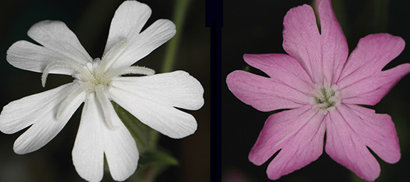
In this challenge we are going to analyse ddRAD data of 12 individuals from two closely related plant species, which were collected at three different sites (A, B, C). (i) Are these two species genetically differentiated and (ii) is there evidence for hybridization? The ddRAD data contains 1000 simulated loci including potential sequencing errors. The average fragment size was 500 bp and the library was sequenced using an 100 bp single-end protocol. The data is already demultiplexed (barcode with 5 characters). There is no reference genome available so we have to use dDocent in the de novo mode.
De novo assembly, read mapping and SNP calling using dDocent
We are going to use the interactive pipeline of dDocent.
If you have your own data I would highly recommend to go through dDocent step by step, there is a good tutorial available on Github.
Login to our server.
ssh studentX@gdcsrv2.ethz.ch
First, we have to load the dDocent software package.
module load dDocent/v2.2.25
Let's generate a folder, download the data and extract the files.
mkdir RAD
cd RAD
wget https://www.gdc-docs.ethz.ch/GeneticDiversityAnalysis/GDA20/data/RAD.tar.gz
tar xvzf RAD.tar.gz
ls
As you can see there are 12 single-end fastq files. Let's execute dDocent by typing
dDocent
It searches first for the fastq files. You have to verify the number of found fastq files.
yes
[ENTER]
Now, you have to select the number of CPUs, since we are many people we set it to 2.
2
Please enter the maximum memory to use for this analysis. Let's say 5 GB.
5g
Next, we have to confirm that you want to trim the data.
yes
[ENTER]
Then, we want to perform an assembly using only single-end reads.
yes
[ENTER]
SE
[ENTER]
Then, we have to define the similarity to cluster. That depends on the divergence of the species. We are using here the default parameters (0.90).
no
[ENTER]
Now, we have to confirm that we want to map the reads using the standard parameters.
yes
[ENTER]
no
[ENTER]
The last step is now to call the SNPs using FreeBayes. You don't have to fill in your email.
yes
[ENTER]
The pre clustering will take only a few seconds and now, we have to set a data cutoff. Normally, I would not be too stringent here, let's say that the sequence has to be covered at least by 3 reads across all individuals. We can be more stringent during the filtering procedure.
3
[ENTER]
As suggested we set the second parameter to 2 meaning that the sequence has to be present in 2 of the 12 individuals.
2
[ENTER]
The program would run for about 10 min. To save time we now quite the process (CTRL-C). Find the outputs already in your working directory. Since the data files are pretty small you get a warning information about raw.*.vcf, just ignore it.
(1)Try to recall the different steps of the pipeline.

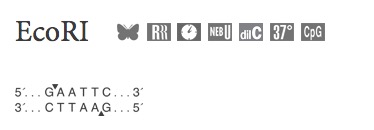
(2) Which restriction enzymes has been used? Have a look at one of the fastq files. First, you can count the number of reads. Then, the combination of grep and wc -l helps you to check if a certain sequence AAA is present in all sequences (remember RegEx). Then, you can quickly google the sequence.
less A_1.F.fq.gz
Suggestion
##number of reads
zcat A_1.F.fq.gz |grep "^@" | wc -l

##how many reads start with AA.....
zcat A_1.F.fq.gz|grep "^AA"|wc -l
zcat A_1.F.fq.gz|grep "^AAT"|wc -l
zcat A_1.F.fq.gz|grep "^AATT"|wc -l
zcat A_1.F.fq.gz|grep "^AATTC"|wc -l
zcat A_1.F.fq.gz|grep "^AATTCC"|wc -l
(3) Have a look at the de novo assembly (reference.fasta). How many fragments do you have in your catalogue ? Here we have simulated data and we know the expected number. How good was our de novo assembly and which parameters might influence the catalogue size? How many mismatches per fragment have you allowed with the used clustering parameter?
Suggestions
## Number of fragments in the catalogue
grep ">" reference.fasta| wc -l
95 bp reads (100 - 5 (barcode))
95/100*10 ~9.5 bp differences among the reads
If you have empirical data, you have to run the script with different parameters to find an optimum.
SNP table filtering
Although, we have filtered already SNP tables, filtering is important especially with RAD data. We will systemically filter our generated SNP table. We are going to use TotalSNPs.vcf. dDocent outputs also a filtered vcf file (Final.recode.vcf), which we can then use for comparison.
First, have a look at the total numbers of SNPs, the number of rows in a vcf file represents the number of SNPs but we have to exclude the lines starting with #.
cat TotalRawSNPs.vcf| grep -v '^#' | wc -l
Now, we will keep only sites with a quality score of larger than 20. The minor allele count we set to 3 and for many population genetic analyses we need to remove low frequency alleles. Let's say we only consider alleles that are present in at least 5% of the individuals.
vcftools --vcf TotalRawSNPs.vcf --minQ 20 --mac 3 --maf 0.05 --recode --recode-INFO-all --out raw_20_mac3_maf5
(1) How many SNPs are retained ?
What is the mean coverage per site? We are going to compute the mean depth per site and plot the histogram directly in the terminal. First, we calculate the mean depth using VCFtools and extract the mean depth per site and divide these numbers by the number of individuals (12 in our case) and then plot the data.
vcftools --vcf raw_20_mac3_maf5.recode.vcf --site-depth
cut -f3 out.ldepth | awk -v x=12 '{print $1/x}' > meandepthpersite

gnuplot << \EOF
set terminal dumb size 120, 30
set autoscale
set xrange [5:30]
unset label
set title "Histogram of mean depth per site"
set ylabel "Number of Occurrences"
set xlabel "Mean Depth"
binwidth=1
bin(x,width)=width*floor(x/width) + binwidth/2.0
set xtics 5
plot 'meandepthpersite' using (bin($1,binwidth)):(1.0) smooth freq with boxes
pause -1
EOF
As you can see the depth is normally distributed around 18 X (with empirical data the distribution looks much more skewed). We set the mean depth to 15, the minimum depth to 6 and the maximum to 25. These numbers remain, however, arbitrary you can also test other combinations. In the current version of dDocent there is even a more sophisticated coverage filtering method implemented.
vcftools --vcf raw_20_mac3_maf5.recode.vcf --minDP 6 --min-meanDP 15 --max-meanDP 30 --recode --recode-INFO-all --out raw_20_mac3_maf5_minDP6_meanDP15_maxDP25
(2) How many SNPs are retained?
Now, we want to exclude sites with too many missing data. There are maybe samples with many missing genotypes. We first calculate the number of missing sites using VCFtools. Based on the output file (out.imiss) you can choose which individual(s) need to be removed.
vcftools --vcf raw_20_mac3_maf5_minDP6_meanDP15_maxDP25.recode.vcf --missing-indv
(3) Are there sample(s) that we have to exclude?
We now generate a list including individual(s) that needs to be removed. Please replace XXX with the respective individual(s).
echo "XXX" >  miss_Ind.txt
vcftools --vcf raw_20_mac3_maf5_minDP6_meanDP15_maxDP25.recode.vcf --remove miss_Ind.txt --recode --recode-INFO-all --out raw_20_mac3_maf5_minDP6_meanDP15_maxDP25_reduced
The next step is to filter sites > 10% missing genotypes. We cannot directly use the --max-missing option of VCFtools because we would like that all three sites are equally represented with < 10% missing genotypes each. First, we are going to generate a list of individuals for each population. dDocent has generated already by default a population map based on the name of the fastq files (Pop_individual.F.fq.gz). We just need to split the popmap into 3 parts (popA, popB, popC). We then calculate the number of missing sites per population. These three files will be concatenated, headers removed, and we select loci with > 0.1 missing data and save these loci and position in the file badloci. We then remove these badloci from the vcf file.
awk '$2 == "A"' popmap > popA
awk '$2 == "B"' popmap > popB
awk '$2 == "C"' popmap > popC
vcftools --vcf raw_20_mac3_maf5_minDP6_meanDP15_maxDP25_reduced.recode.vcf --keep popA --missing-site --out A
vcftools --vcf raw_20_mac3_maf5_minDP6_meanDP15_maxDP25_reduced.recode.vcf --keep popB --missing-site --out B
vcftools --vcf raw_20_mac3_maf5_minDP6_meanDP15_maxDP25_reduced.recode.vcf --keep popC --missing-site --out C
cat A.lmiss B.lmiss C.lmiss | awk '!/CHR/' | awk '$6 > 0.1' | cut -f1,2  > badloci

vcftools --vcf  raw_20_mac3_maf5_minDP6_meanDP15_maxDP25_reduced.recode.vcf --exclude-positions badloci --recode --recode-INFO-all --out raw_20_mac3_maf5_minDP6_meanDP15_maxDP25_reduced_NA10
(4) What is the final number of SNPs? Ddocent has also generated a vcf file (Final.recode.vcf). How many SNPs are retained here?
Here we have only simulated data and stop at this point.
There are even more filter criteria like mapping qualities between reference and alternate alleles, a quality score below ¼ of the depth and the observed allele frequencies in the population or Hardy-Weinberg equilibrium. You find more detailed information in the tutorial of dDocent. Normally, people also remove indels and often decompose complex SNPs using vcfallelicprimitives since for most downstream analyses only single SNPs could be considered. For many population genetic analyses such as STRUCTURE you need unlinked loci. One possibility is to randomly choose one locus per fragment alternatively you can haplotype your ddRAD data using rad_haplotyper, which allows you also to filter paralogous loci in your assembly.
Visualization
We have filtered our SNP table now we want to visualize the data. To get a first impression of the global picture we are performing a Principal Component Analysis (PCA). We are going to execute the R script directly in the terminal (PCA_vcf.R). To run an R-script on the command-line in order to generate a PCA and produce a pdf you just need to call the script with your filtered vcf file and the population information.
Rscript PCA_vcf.R "raw_20_mac3_maf5_minDP6_meanDP15_maxDP25_reduced_NA10.recode.vcf" "popmap"
(1) Try to understand the Rscript as we execute the R script directly in the terminal.
(2) Can you identify the two species? Are there any hybrids? How representative is this plot? Do you see differences regarding the different version of your vcf file?
(3) Let's try to quantify the differences between the two species using for example Fst, VCFtools has the function implemented. For more information have a look at the manual page here. Use then R to plot the Fst values.
Suggestion
vcftools --vcf raw_20_mac3_maf5_minDP6_meanDP15_maxDP25_reduced_NA10.recode.vcf --weir-fst-pop popA --weir-fst-pop popB
fst <- read.table("out.weir.fst", header=T)
boxplot(fst$WEIR_AND_COCKERHAM_FST)
hist(fst$WEIR_AND_COCKERHAM_FST)
RAD tags simulations
In case you like to use RADseq the first step is to decide which restriction enzymes to like to use. To get an idea how many fragments you get for your restriction enzymes you can do an in silco digest using your genome of interst or from a closely related species. Here we will simulate a genome.
SimRAD provides a number of functions to simulate restriction enzyme digestion, library construction and fragments size selection to predict the number of loci expected from most of the Restriction site Associated DNA (RAD) and Genotyping By Sequencing (GBS) approaches. SimRAD aims to provide an estimation of the number of loci expected from a given genome depending on protocol type and parameters allowing to assess feasibility, multiplexing capacity and the amount of sequencing required.
(1) Install "Biostrings" and "ShortRead" from bioconductor and the SimRAD package. Load then the package to make sure that it has been installed successfully.
if (!requireNamespace("BiocManager"))
    install.packages("BiocManager")
BiocManager::install(c("Biostrings", "ShortRead"))

install.packages("SimRAD",dependencies=T)
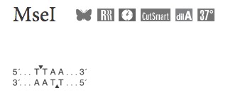
(2) From the manual we got the following code. The task is now to modify it as following: We are going to simulate 100,000 bp genome, use EcoRI and TaqI and select a range of 330-430. Find the information about the restriction enzymes below. How many fragments do you predict?
#Restriction Enzyme 1
#TaqI
cs_5p1 = "T"; cs_3p1 = "CGA"
#Restriction Enzyme 2
#MseI #
cs_5p2 = "T"; cs_3p2 = "TAA"

#simulate a genome
simseq<-sim.DNAseq(size=10000, GCfreq=0.51)

#digest the genome
simseq.dig<-insilico.digest(simseq, cs_5p1, cs_3p1, cs_5p2, cs_3p2, verbose=TRUE)

#select appropriate fragmnets
simseq.sel<-adapt.select(simseq.dig, type="AB+BA", cs_5p1,cs_3p1, cs_5p2, cs_3p2)

# wide size selection (200-270):
wid.simseq<-size.select(simseq.sel,min.size = 200,max.size = 270,graph=TRUE,verbose=TRUE)
Suggestion
library(SimRAD)
# Restriction Enzyme 1
# EcoRI #
cs_5p1 <- "G"
cs_3p1 <- "AATTC"
# Restriction Enzyme 2
# TaqI
cs_5p2 <- "T"
cs_3p2 <- "CGA"

# simulate a genome
simseq <- sim.DNAseq(size = 1000000, GCfreq = 0.51)

# digest the genome
simseq.dig <- insilico.digest(simseq, cs_5p1, cs_3p1, cs_5p2, cs_3p2, verbose = TRUE)

# select appropriate fragmnets
simseq.sel <- adapt.select(simseq.dig, type = "AB+BA", cs_5p1, cs_3p1, cs_5p2, cs_3p2)

# wide size selection (200-270):
wid.simseq <- size.select(simseq.sel, min.size = 330, max.size = 430, graph = T, verbose = T)
(3) How many fragments do you predict for a 500 Mbp genome?
Suggestion
500000000 / 100000 * 32