RNA-Seq
Lecture Notes
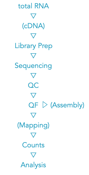
⬇︎ RNA-Seq
RNA-sequencing analyzes the transcriptome. Some of the most popular techniques are transcriptional (expression) profiling, differential gene expression analysis, RNA editing and even SNP identification. We will focus on the analysis to identify differential expressed genes (DEGs). There are many methods but no consensus about the most appropriate workflow to identifying differentially expressed genes from RNA-Seq data. Have a look at Costa-Silva et. al (2017) for am extended review on the topic.
Quality Control
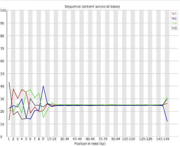
Content Bias - Depending on the library preparation method, QC of RNA-Seq data sets often show a pronounced sequence composition bias at the beginning (first ~12 bases) of the reads. The origin of this bias is related to the random priming step in the library production. The priming should be equal efficiency for all hexamer primers, which is not the case. Trimming the reads would remove the (visual) bias, but it would be wrong and not solve the problem. The QC warning is correct, but there is not much you can / should do.
Contaminations - Getting high-quality intact total RNA is often the first step in many biological applications aimed at measuring gene expression. A tough task and it is not uncommon to sequences short fragments. Keep an eye open for adaptor contamination.
With the careful extraction of RNA we are not only isolating mRNA but other RNA molecules. Some library preparation workflows include a ribosomal RNA depletion step.
Duplicate Sequences - Nothing to worry about. We expect high(er) level of duplication in RNA-Seq datasets. Specific enrichments is a characteristic of RNA-Seq and does not indicating over-sequencing. A de-duplication step would remove the expression signal.
RNA Integrity
A QC like provided with FastQC does not reflect the true quality of RNA-Seq data. You might consider transcript integrity number (TIN) score PCA plot to infer the true quality (Son et al. 2018).
Data Filtering
With the careful extraction of RNA we are not only isolating mRNA but other RNA molecules. Some library preparation workflows include a ribosomal RNA depletion step.
Approximately 80 percent of the total RNA in rapidly growing mammalian cells (e.g., cultured HeLa cells) is rRNA, and 15 percent is tRNA; protein-coding mRNA thus constitutes only a small portion of the total RNA. The primary transcripts produced from most rRNA genes and from tRNA genes, like pre-mRNAs, are extensively processed to yield the mature, functional forms of these RNAs. < Molecular Cell Biology>
Therefore, it is important to screen (and filter) the sequence reads for non mRNA related data. A convenient screen application would be FastQ Screen
Statistical Power of RNA-seq Experiments
First, we run a few sample-size power simulation in R using either RNASeqPower or PROPER. Both are Bioconductor packages and can be installed via the BiocManager.
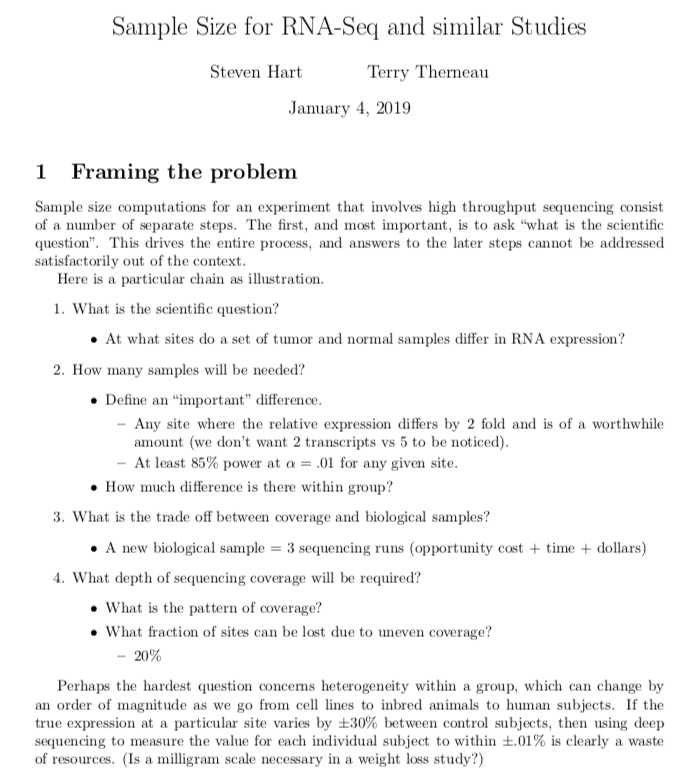
In the short manual of RNASeqPower Steven Hart and Terry Therneau do a wonderful job describing the problems of the experimental design of an RNA-seq experiment.
Exercise: Power Analysis
For the RNA-Seq exercise, we focus on the data analysis in R. First you have to download the R script first. You have two choices. Either you are using the wget command to download the R script to your local hard drive and open it with RStudio or you download and open the script directly within RStudio. Choose the one you prefer or try both to compare.
Terminal
## Working Directory
mkdir ${HOME}/RNASeq
cd ${HOME}/RNASeq

## Get R script via terminal
wget "http://www.gdc-docs.ethz.ch/GeneticDiversityAnalysis/GDA20/scripts/PowerAnalysis.R"
RStudio
## --------------------------------
## Get R script via R console
## --------------------------------

# We use wget from the HelpersMG package.
# Check if you have the package already installed:
# installed.packages(HelpersMG)
# If not, you have to install the package:
# install.packages("HelpersMG")

library("HelpersMG")

## Working Directory
getwd()                # current directory
#setwd()               # set directroy if needed
dir.create("RNASeq")   # new working directory
setwd("RNASeq")        # ready to go

## Downlaod R script
wget("http://www.gdc-docs.ethz.ch/GeneticDiversityAnalysis/GDA20/scripts/PowerAnalysis.R")

## Open the script
file.edit("PowerAnalysis.R")
The benefit of power analysis might debatable, but these simulations help to understand the importance of biological replicates. Therefore, it is essential that you are not just copy and paste the code but understand it.
Tip
RNA-Seq experiments are powerful if well designed but limited if not. The within sample variations has to be low or the number of replicates (very) high if you want to trust in the results of your differential expression study.
RNA-Seq Data Analysis
Exercise: DESeq2
◇ Special thanks to Heidi E.L. Tschanz-Lischer
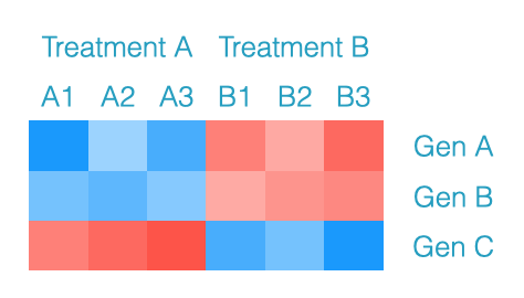
The next exercise is a step-by-step RNA-Seq analysis to find differential expression genes in newborn (N), juvenile (J) and adult (A) mice. Male and females from all life-stages were sequenced.
## Download the Count Table
library(HelpersMG)
wget("http://www.gdc-docs.ethz.ch/GeneticDiversityAnalysis/GDA20/data/RNAseq_Mus.txt")

## Import Count Table
countTable <- read.delim("RNAseq_Mus.txt", header = TRUE, row.names = 1)

## Data format
head(countTable)
# ENSMUSG - Ensemble Mouse (Mus musculus) Genome
# Example:
# ENSMUSG00000020333 > Acsl6 (acyl-CoA synthetase long-chain family member 6)
# This gene has 15 transcripts (splice variants), 161 orthologues, and 13 paralogues.
# f/m = female/male; N/J/A: newborn/juvenile/adults
We need a sample-design table:
group <- data.frame(condition = c("N","N","J","J","A","A"),
                    sex = c("f","m","f","m","f","m"),
                    row.names = names(countTable))
group
We are using the Bioconductor package DESeq2 to find DEGs.
## Installed DESeq2
# if (!requireNamespace("BiocManager", quietly = TRUE))
#    install.packages("BiocManager")

BiocManager::install("DESeq2")
# > This might take a while since DESeq2 depends on other libraries.

## Load Library
library(DESeq2); packageVersion("DESeq2")

## DESeq Data Set
dds <- DESeqDataSetFromMatrix(
                 countData = countTable,
                 colData   = group,
                 design    = ~sex + condition)
Plot a PCA & Clusters of log2 transformed normalized counts to check for outliers.
## Regularized Log Transformation
rld   <- rlog(dds, blind = FALSE)
dist  <- dist(t(assay(rld)))
hc    <- hclust(dist)

## PCA Plot
plotPCA(rld)

## Cluster
plot(hc)

⟹  No outliers, m & f (replicates) of the same age group together.
⟹  Newborn and juvenile are more similar.
The standard differential expression analysis steps are all wrapped into a single function: DESeq. To get differentially expressed genes between e.g. newborns and adults you need to execute following commands:
# Standard Analysis
deg    <- DESeq(dds)
res.NA <- results(deg, contrast = c("condition", "N", "A"))
res.JA <- results(deg, contrast = c("condition", "J", "A"))
res.NJ <- results(deg, contrast = c("condition", "N", "J"))

# Results
head(res.NA)
# Meaning
mcols(res.NA)$description

# => e.g. Acsl6 (ENSMUSG00000020333) is not significantly different expressed between newborn and adults.
#                                    is significantly different expressed between juvenile and adults.
#                                    is not significantly different expressed between newborn and juvenile.
The DESeq function performs following steps, which can be run manually:
# Normalize the count data set by estimating the size factor:
esf <- estimateSizeFactors(dds)

# If each column of the count table is divided by the size factor for this column,
# the count values are brought to a common scale.
# To view the size Factors you can execute following command:
sizeFactors(esf)

# Estimate variance (dispersion) of gene expression between biological replicates.
# We use M and F as biological replicates

# If the gene expression differs between replicates by 20%, then the gene’s dispersion is 0.2^2 = 0.04.
disp <- estimateDispersions(esf)

# Plot extimated variance (red line= fitted dispersion):
plotDispEsts(disp)

# Get differentially expressed genes:
deg.manual <- nbinomWaldTest(disp)
DEGs with adjusted p-value cutoff (FDR) < 5%:
## Results
summary(res.NA, alpha = 0.05)
summary(res.JA, alpha = 0.05)
summary(res.NJ, alpha = 0.05)

# Plot all DEGs (FDR < 5% in red):

par(mfrow = c(3,1))
 plotMA(res.NA, alpha = 0.05, main = "Newborn-Adult")
 plotMA(res.JA, alpha = 0.05, main = "Juvenile-Adult")
 plotMA(res.NJ, alpha = 0.05, main = "Newborn-Juvenile")
par(mfrow = c(1,1))
Individual DEGs:
# Plot normalized counts for a single gene
plotCounts(dds, gene = "ENSMUSG00000020333")

# Plot count of the most significant DEG for N-A:
plotCounts(dds, gene = which.min(res.NA$padj))
# res.NA[which.min(res.NA$padj),]
# ⟹  ENSMUSG00000054932: Afp (alpha-foetoprotein - plasma protein)

# Plot count of the most significant DEG for J-A:
plotCounts(dds, gene = which.min(res.JA$padj))
# res.JA[which.min(res.JA$padj),]
# ⟹  ENSMUSG00000005547: Cyp2a5 (cytochrome P450)

# Plot count of the most significant DEG for N-J:
plotCounts(dds, gene = which.min(res.NJ$padj))
# res.NJ[which.min(res.NJ$padj),]
# ⟹  ENSMUSG00000032517: Mobp (myelin-associated oligodendrocytic basic protein)

# Order results according strength of differential expression:
res.NA.ordered <- res.NA[order(res.NA$padj), ]
Get list of over-expressed genes in newborns/adults at FDR 5%:
## over-expressed genes in N (bigger 0)
overN <- res.NA.ordered[res.NA.ordered$padj < 0.05 & !
is.na(res.NA.ordered$padj) & res.NA.ordered$log2FoldChange > 0, ]
nrow(overN)

## over-expressed genes in A (smaller 0)
overA <- res.NA.ordered[res.NA.ordered$padj < 0.05 & !
is.na(res.NA.ordered$padj) & res.NA.ordered$log2FoldChange < 0, ]
nrow(overA)
Write differential expression table in a text file:
write.table(res.NA.ordered, "DEGs_Newborn_Adults.txt", sep = "\t", row.names = TRUE)
The Bioconductor BiomaRt R package is a quick, easy and powerful way to access BioMart right from your R software terminal.
# if (!requireNamespace("BiocManager", quietly = TRUE))
#    install.packages("BiocManager")
# BiocManager::install("biomaRt")

library(biomaRt)

## Available Datasets
# mart = useEnsembl('ENSEMBL_MART_ENSEMBL')
# listDatasets(mart)

ensembl = useEnsembl(biomart="ensembl", dataset="mmusculus_gene_ensembl")

## Available Attributes
# listAttributes(ensembl)

## Dataset for Mouse Genome
genes <- getBM(attributes=c('ensembl_gene_id',
                            'ensembl_transcript_id',
                            'description',
                            'external_gene_name'
                            'chromosome_name',
                            'start_position',
                            'end_position'),
                            filters = 'chromosome_name', values = c(1:20), mart = ensembl)

# Gene Name
unique(genes$external_gene_name[genes$ensembl_gene_id == "ENSMUSG00000032517"])
# Gene description
unique(genes$description[genes$ensembl_gene_id == "ENSMUSG00000032517"])
# Chromosome
unique(genes$chromosome_name[genes$ensembl_gene_id == "ENSMUSG00000032517"])
Additional Information
Analysis Workflows
RNA-Seq News / Infos
Evaluation of RNA-Seq data quality
Read-Mappers
Super-Fast alternative to conventional Read-Mappers:
Mapping-Viewer
Literature
- Conesa et al. (2016) A survey of best practices for RNA-seq data analysis.
- Costa-Silva et al. (2017) RNA-Seq differential expression analysis: An extended review and a software tool.
- Hansen et al. (2010) Biases in Illumina transcriptome sequencing caused by random hexamer priming.
- Son et al. (2018) A simple guideline to assess the characteristics of RNA-Seq data.